Hamiltonian Mechanics: From Velocities to Momenta

At the end of the last topic, I asked you to sit with an unresolved suspicion: why is the Lagrangian $\mathcal{L} = T - V$ , kinetic minus potential, rather than $T + V$ , the total energy — a quantity you already understood perfectly well before any of this started? I promised the answer would be more interesting than a hand-wave. Here it is, and it requires one more reformulation.

A question worth asking before diving in

Lagrangian mechanics already solved the constraint-force problem beautifully — why mess with a working formula? Here's a concrete reason: the Euler-Lagrange equation is second-order in time (it has $\ddot{q}$ buried inside $\frac{d}{dt}\frac{\partial\mathcal{L}}{\partial\dot q}$ ). Second-order equations are more awkward to work with than first-order ones — in numerical simulation, in proving general theorems about the structure of mechanics, and, as we're about to see, in building a bridge to quantum theory. So the question is: can we trade in $\ddot q$ for something and end up with two first-order equations instead of one second-order one?

Generalized momentum

Define, for each generalized coordinate $q_i$ , its conjugate momentum:

p_i = \frac{\partial \mathcal{L}}{\partial \dot{q}_i}

For an ordinary particle in Cartesian coordinates, this reproduces the momentum you already know: $\mathcal{L} = \frac{1}{2}m\dot x^2 - V(x)$ gives $p = m\dot x$ , the familiar $p = mv$ . But the definition is more general than that — in other coordinate systems, "momentum" conjugate to an angle, for instance, turns out to be angular momentum, entirely for free, just from applying the same formula.

The Legendre transform: swapping variables

Here's the actual trick. Define a new function, the Hamiltonian, built from the Lagrangian by:

H(q, p) = \sum_i p_i \dot{q}_i - \mathcal{L}(q, \dot{q})

This construction — take a function of one variable, and re-express it as a function of that variable's own "slope" instead — is called a Legendre transform, and it's the same piece of mathematical machinery that connects several pairs of quantities in thermodynamics. Mechanically, what it does here is subtle but important: $H$ is defined so that once you substitute $\dot q_i \to p_i$ everywhere (using $p_i = \partial\mathcal L/\partial\dot q_i$ , inverted to solve for $\dot q_i$ in terms of $p_i$ ), the velocity disappears completely, and $H$ becomes a function purely of position and momentum.

Let's just try it on the simplest possible system and see what falls out. A free particle under a potential: $\mathcal{L} = \frac{1}{2}m\dot x^2 - V(x)$ . We already have $p = m\dot x$ , so $\dot x = p/m$ . Substitute into the definition of $H$ :

H = p\dot x - \mathcal{L} = p\left(\frac{p}{m}\right) - \left[\frac{1}{2}m\left(\frac{p}{m}\right)^2 - V(x)\right] = \frac{p^2}{m} - \frac{p^2}{2m} + V(x) = \frac{p^2}{2m} + V(x)

And there's the resolution I promised. $\frac{p^2}{2m}$ is kinetic energy, expressed in momentum instead of velocity, and $V(x)$ is potential energy — so $H = T + V$ , the total mechanical energy, exactly the quantity your instinct wanted the Lagrangian to be all along. The Lagrangian and the Hamiltonian aren't in conflict; they're a Legendre-transform pair, related by exactly the algebra above, and each is the natural energy-like quantity for a different choice of variables — $(q,\dot q)$ for one, $(q,p)$ for the other.

Hamilton's equations

Carrying the Legendre transform through the Euler-Lagrange equation carefully (a short exercise in the chain rule, which we won't belabor here) produces Hamilton's equations:

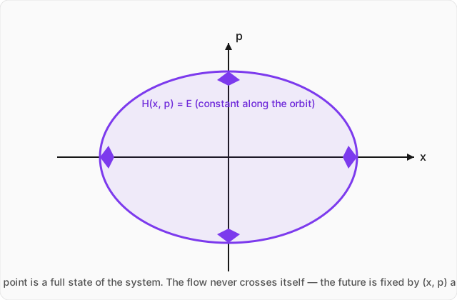
\dot{q}_i = \frac{\partial H}{\partial p_i} \qquad \dot{p}_i = -\frac{\partial H}{\partial q_i}

Two first-order equations where before there was one second-order equation — exactly the trade we set out to make. They also reveal a strikingly symmetric structure between position and momentum that's completely invisible in the Lagrangian formulation, where $q$ and $\dot q$ play very different grammatical roles. Here, $q$ and $p$ are treated on almost equal footing, living together as coordinates of a single space called phase space: at any instant, the pair $(q,p)$ is the entire state of the system — nothing about the past matters beyond what's encoded in that one point, and nothing about the future is undetermined once you have it.

A closed elliptical orbit in the x-p phase plane, with arrows showing clockwise flow, representing a system of constant Hamiltonian H equals E. — A trajectory in phase space for a system with constant energy. Because the state (x, p) fully determines the future, phase-space trajectories can never cross themselves.

Worked example

Find Hamilton's equations for a mass m on a spring of constant k, and show they reproduce simple harmonic motion. (click to reveal the solution)

The Lagrangian: with position $x$ , $\mathcal{L} = \frac{1}{2}m\dot x^2 - \frac{1}{2}kx^2$ .

Conjugate momentum:

p = \frac{\partial \mathcal{L}}{\partial \dot x} = m\dot x \quad\Longrightarrow\quad \dot x = \frac{p}{m}

The Hamiltonian, via the Legendre transform (same steps as the free-particle case above, with $V(x) = \frac{1}{2}kx^2$ ):

H = \frac{p^2}{2m} + \frac{1}{2}kx^2

— total energy, exactly as it should be for a system where energy is conserved.

Hamilton's equations:

\dot x = \frac{\partial H}{\partial p} = \frac{p}{m} \qquad\qquad \dot p = -\frac{\partial H}{\partial x} = -kx

Recovering the familiar equation: differentiate the first equation with respect to time, $\ddot x = \dot p / m$ , then substitute the second equation:

\ddot x = \frac{-kx}{m} = -\frac{k}{m}x

— exactly the simple harmonic oscillator equation. Two clean first-order equations gave us back the one second-order equation we'd have written down directly from Newton's second law, but along the way we picked up the phase-space picture in the figure above: this system traces a closed ellipse in the $(x,p)$ plane, over and over, forever, because $H = E$ never changes.

Where this leads

Here's the payoff for all this restructuring, and it's a genuinely remarkable fact about how nature is built. The specific algebraic structure of Hamilton's equations — the particular way $q$ and $p$ pair up and trade off against each other — turns out to be exactly the classical shadow of the mathematical structure underlying quantum mechanics. The step from here to there involves promoting $q$ and $p$ from numbers to operators, and Hamilton's equations become, almost unchanged in form, the equations that govern how a quantum state evolves in time. Physicists usually describe this as "quantizing" a classical system — and it's a far shorter step from a Hamiltonian than it would ever be from a bare Newtonian force law. That step, and everything on the other side of it, is where this track goes next: into quantum mechanics.