Lagrangian Mechanics: Reformulating Newton

Try this with what you already know. A pendulum swings on a rigid rod from a fixed pivot. Write down $\vec{F} = m\vec{a}$ for the bob.

Go ahead — you'll immediately hit a snag that Newton's laws never warned you about. The rod exerts a tension force on the bob, constantly changing direction and magnitude as the pendulum swings, doing exactly whatever is necessary to keep the bob at a fixed distance from the pivot. You don't actually care about that tension — you want the bob's motion, not the rod's internal stress — but $\vec{F} = m\vec{a}$ in ordinary $x,y$ coordinates forces you to solve for it anyway, just to eliminate it from the equations afterward. It's a lot of unwanted bookkeeping for a system that, intuitively, has only one real degree of freedom: the swing angle.

This is not a one-off annoyance. It's the generic situation whenever motion is constrained — a bead on a curved wire, a block on a wedge that's itself free to slide, two masses connected by a rope over a pulley. Every one of these has some hidden force doing invisible bookkeeping work, and Newton's framework makes you compute it whether you want it or not. So the honest question is: is there a way to write down the physics that never mentions the constraint force in the first place?

There is. It requires walking away from force vectors almost entirely, in favor of a single scalar function. That trade turns out to be one of the most productive moves in the history of physics — work and energy already showed you a taste of what thinking in scalars, instead of vectors, can buy you, and this is that idea taken all the way.

Generalized coordinates: describe the freedom, not the space

Instead of Cartesian $x, y$ , describe a system's configuration with generalized coordinates $q_1, \ldots, q_n$ — one for each true degree of freedom the system actually has. For the pendulum, that's just one number: the angle $\theta$ .

A pendulum hanging from a pivot, showing the swing angle theta, with dashed lines showing how the bob's Cartesian x and y coordinates are both determined by that single angle. — The bob's Cartesian position needs two numbers (x, y) constrained by x² + y² = L². Its actual freedom to move needs exactly one: θ.

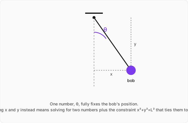
Watch what just happened: the constraint that made Newton's approach painful — the fixed rod length — has been built directly into the choice of coordinate. There's no leftover tension force to solve for, because $\theta$ already respects the constraint by construction. This is the whole strategy of Lagrangian mechanics in one picture.

The Lagrangian: kinetic minus potential

Define a single scalar function, the Lagrangian, as kinetic energy minus potential energy:

\mathcal{L} = T - V

It's fair to be suspicious of this. Kinetic minus potential, rather than their sum — which would just be total energy, a quantity you already understand? Hold that suspicion; it won't resolve until the next section, and it's worth not letting it resolve prematurely, because the resolution is more interesting than any hand-wave I could offer you now.

The Principle of Least Action

Define the action as the time-integral of the Lagrangian along some candidate path the system might take between two fixed configurations:

S = \int_{t_1}^{t_2} \mathcal{L}(q, \dot{q}, t)\, dt

Here is the claim, and it is a genuinely strange one the first time you meet it: of every conceivable path a system could take between a starting configuration and an ending configuration, the one it actually takes is the one that makes $S$ stationary — an extremum, almost always a minimum — compared to all the others. Nature, in some sense, is comparing an infinity of hypothetical trajectories and selecting the one with the least action.

This is a wildly different picture of causation than "a force pushes it, so it accelerates, instant by instant." It's not obviously equivalent to that picture either — which is exactly why it's worth deriving the consequence explicitly rather than taking it on faith.

The Euler-Lagrange equation

Grinding through the calculus of variations to make $S$ stationary — perturb the path slightly, demand the first-order change in $S$ vanishes, integrate by parts — produces, for each generalized coordinate $q_i$ , the Euler-Lagrange equation:

\frac{d}{dt}\left(\frac{\partial \mathcal{L}}{\partial \dot{q}_i}\right) - \frac{\partial \mathcal{L}}{\partial q_i} = 0

This one template, applied once per degree of freedom, replaces the entire ritual of free-body diagrams and force components. Write $T$ and $V$ in your generalized coordinate, form $\mathcal{L} = T - V$ , apply this formula, and the equation of motion falls out — constraint forces never appear, because a constraint force, by definition, does no work in the direction the constraint forbids, and this formalism only ever asks about the directions the system is actually free to move in.

Sanity check: does it reproduce Newton?

Before trusting this machine on the pendulum, make sure it doesn't disagree with what you already know. For a free particle of mass $m$ in one Cartesian dimension $x$ , under potential $V(x)$ : $T = \frac{1}{2}m\dot{x}^2$ , so $\mathcal{L} = \frac{1}{2}m\dot{x}^2 - V(x)$ . Then $\frac{\partial \mathcal{L}}{\partial \dot{x}} = m\dot{x}$ and $\frac{\partial \mathcal{L}}{\partial x} = -\frac{\partial V}{\partial x}$ . Substituting into the Euler-Lagrange equation:

\frac{d}{dt}(m\dot{x}) + \frac{\partial V}{\partial x} = 0 \quad\Longrightarrow\quad m\ddot{x} = -\frac{\partial V}{\partial x} = F

using the conservative-force relationship from the work-energy topic. Straight back to $F = ma$ . Nothing was lost — and, as the pendulum is about to show, a great deal is about to be gained.

Worked example

Use the Euler-Lagrange equation to find the equation of motion of a simple pendulum: a bob of mass m on a rigid, massless rod of length L, swinging under gravity. (click to reveal the solution)

Setting up: One degree of freedom, the angle $\theta$ from vertical (as in the figure above). The bob's Cartesian position is $x = L\sin\theta$ , $y = -L\cos\theta$ , so its speed is:

\dot{x}^2 + \dot{y}^2 = L^2\dot\theta^2\cos^2\theta + L^2\dot\theta^2\sin^2\theta = L^2\dot\theta^2

Kinetic and potential energy, taking the lowest point of the swing as the reference height:

T = \frac{1}{2}mL^2\dot\theta^2 \qquad V = mgL(1-\cos\theta)

The Lagrangian:

\mathcal{L} = T - V = \frac{1}{2}mL^2\dot\theta^2 - mgL(1-\cos\theta)

Applying the Euler-Lagrange equation. First the momentum-like term:

\frac{\partial \mathcal{L}}{\partial \dot\theta} = mL^2\dot\theta \quad\Longrightarrow\quad \frac{d}{dt}\left(\frac{\partial \mathcal{L}}{\partial \dot\theta}\right) = mL^2\ddot\theta

Then the other term:

\frac{\partial \mathcal{L}}{\partial \theta} = -mgL\sin\theta

Putting them together:

mL^2\ddot\theta - (-mgL\sin\theta) = 0 \quad\Longrightarrow\quad \ddot\theta = -\frac{g}{L}\sin\theta

That's the pendulum equation — and notice what we never once had to compute: the rod's tension. It vanished from the calculation automatically, exactly as promised, because $\theta$ already encoded the constraint. Getting here through $\vec{F} = m\vec{a}$ directly would have meant resolving tension into $x$ and $y$ components at every instant and eliminating it by substitution — the same physics, considerably more arithmetic.

Where this leads

Lagrangian mechanics is not the final destination — it's a bridge. Reorganize it slightly, via a Legendre transform that trades $\dot{q}$ for a new variable called momentum, and you get Hamiltonian mechanics, which describes systems in terms of position and momentum instead of position and velocity. Hamiltonian mechanics, in turn, is the direct classical ancestor of the mathematical structure that quantum mechanics is built on — the step from a classical Hamiltonian to a quantum one turns out to be remarkably short once you're standing here. That's the path this track continues to follow.