Introduction to Quantum Mechanics

Why would we even ask for a new mechanics?

Imagine an electron source aimed at a barrier with two narrow slits. Behind the barrier is a screen that records each arrival as a tiny, localized flash. If the electrons were ordinary classical particles, the prediction would seem obvious: some pass through the left slit, some pass through the right slit, and the screen shows two broad piles aligned with the openings.

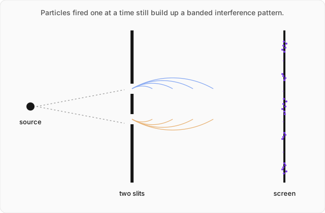
Now reduce the source intensity until the electrons are fired one at a time. Each electron still arrives at one definite point. There is never half an electron on one side of the screen and half on the other. At first the impacts look random. But after hundreds, then thousands, then millions of arrivals, a pattern emerges: alternating bright and dark bands, the unmistakable signature of interference.

That is the puzzle. The electrons arrive like particles, one localized event at a time, but their accumulated distribution behaves like a wave passing through both slits. The pattern remains even when only one electron is in the apparatus at once. There is no second electron with which it could be interfering.

Close either slit and the interference disappears. Open both, and it returns. Try to determine which slit each electron passed through, and the interference is lost. Classical mechanics asks us to assign the electron a trajectory through one slit or the other. The experiment refuses to cooperate.

Description of a double-slit experiment: particles fired one at a time through two slits build up an interference pattern on a screen behind them. — Each impact is localized, but the distribution assembled from many individual impacts contains interference fringes. Quantum mechanics must account for both facts at once.

Cracks in the classical picture

The double-slit experiment is not an isolated trick. By the early twentieth century, several experiments were pointing toward the same uncomfortable conclusion: classical particles and classical waves were not the final categories of nature.

Consider the photoelectric effect. Shine light on a metal and electrons may be ejected. Classical wave theory suggests that making the light more intense should eventually give an electron enough energy to escape, regardless of the light's frequency. Instead, below a threshold frequency, no electrons are emitted, however intense the light becomes.

Einstein proposed that light transfers energy in discrete packets, later called photons. The energy of one packet is

E = hf,

where $f$ is the light frequency and $h$ is Planck's constant. Increasing the intensity supplies more photons, but increasing the frequency increases the energy carried by each photon. Light, the model wave, was behaving in particle-like transactions.

Then de Broglie reversed the question. If light can behave like particles, might matter behave like waves? He associated a wavelength with a particle of momentum $p$ :

\lambda = \frac{h}{p}.

For a baseball, this wavelength is too small to notice. For an electron, it is large enough to produce measurable diffraction and interference. The double-slit pattern is therefore not a decorative analogy. It is evidence that the state of an electron has genuinely wave-like structure.

But we must be careful. An electron is not merely a tiny classical particle riding on a classical wave, nor is it a classical wave smeared through space. What we need is a mathematical framework in which interference and localized detection are both natural consequences.

What becomes of phase space?

Here is where the mechanics you already know becomes useful.

In Hamiltonian mechanics, the state of a one-dimensional particle is represented by a point in phase space. Position $q$ and momentum $p$ live side by side as independent coordinates, and the Hamiltonian $H(q,p)$ determines their evolution through Hamilton's equations:

\dot q = \frac{\partial H}{\partial p}, \qquad \dot p = -\frac{\partial H}{\partial q}.

For a particle of mass $m$ moving in a potential $V(q)$ ,

H(q,p) = \frac{p^2}{2m} + V(q).

Quantum mechanics does not throw this structure away. It changes what the quantities mean.

Position and momentum are promoted from ordinary numbers to operators, $\hat{x}$ and $\hat{p}$ , which act on a state. Unlike classical numbers, these operators do not commute. Their order matters:

[\hat{x},\hat{p}] = \hat{x}\hat{p} - \hat{p}\hat{x} = i\hbar,

where

\hbar = \frac{h}{2\pi}.

This is the quantum resolution of the classical phase-space idea. Classically, one may specify $x$ and $p$ simultaneously and regard them as coordinates of a single point. Quantum mechanically, position and momentum remain the central dynamical variables, but they are noncommuting operators. There is no quantum state corresponding to an arbitrarily sharp classical phase-space point.

The familiar uncertainty relation follows from this operator structure:

\Delta x\,\Delta p \geq \frac{\hbar}{2}.

This is not a claim about clumsy laboratory equipment. It says that no state can possess both an arbitrarily narrow position distribution and an arbitrarily narrow momentum distribution. Classical phase space survives, but not as a set of simultaneously definite values.

The wave function

For a particle moving along one dimension, we describe the state by a complex-valued wave function

\psi(x,t).

The wave function itself is not a directly measured material wave. Its physical meaning enters through the Born rule:

\rho(x,t) = |\psi(x,t)|^2.

Here $|\psi(x,t)|^2$ is the probability density for detecting the particle at position $x$ at time $t$ . Thus the probability of finding it between $a$ and $b$ is

P(a \leq x \leq b) = \int_a^b |\psi(x,t)|^2\,dx.

If the particle is certain to be found somewhere, the wave function must be normalized:

\int_{-\infty}^{\infty} |\psi(x,t)|^2\,dx = 1.

This lets us say precisely what the double-slit experiment displays. The alternatives associated with the two slits contribute amplitudes, not ordinary probabilities. If $\psi_1$ is the amplitude associated with the left slit and $\psi_2$ the amplitude associated with the right slit, then with both slits open,

\psi = \psi_1 + \psi_2.

The observed probability density is therefore

|\psi|^2 = |\psi_1 + \psi_2|^2 = |\psi_1|^2 + |\psi_2|^2 + \psi_1^*\psi_2 + \psi_2^*\psi_1.

The last two terms are the interference terms. They can increase the probability at one location and cancel it at another. If we had merely added classical probabilities, those terms would never appear, and neither would the fringes.

Dynamics: the Schrödinger equation

A state is useful only if we know how it changes. In quantum mechanics, time evolution is governed by the time-dependent Schrödinger equation:

i\hbar\frac{\partial \psi}{\partial t} = \hat{H}\psi.

The operator $\hat{H}$ is the Hamiltonian. This is the point at which the connection to classical mechanics becomes especially satisfying.

For a classical particle in one dimension,

H = \frac{p^2}{2m} + V(x).

For the quantum particle, we use exactly the same Hamiltonian structure, but position and momentum are reinterpreted as operators. In the position representation,

\hat{x} = x, \qquad \hat{p} = -i\hbar\frac{\partial}{\partial x}.

Therefore

\hat{H} = \frac{\hat{p}^{\,2}}{2m} + V(x) = -\frac{\hbar^2}{2m}\frac{\partial^2}{\partial x^2} + V(x).

Substituting this into the Schrödinger equation gives

i\hbar\frac{\partial \psi(x,t)}{\partial t} = -\frac{\hbar^2}{2m}\frac{\partial^2\psi(x,t)}{\partial x^2} + V(x)\psi(x,t).

So the Hamiltonian you met in classical mechanics has not vanished. It is still the generator of time evolution. The expression

H = \frac{p^2}{2m} + V(x)

becomes

\hat{H} = \frac{\hat{p}^{\,2}}{2m} + V(x),

with $p$ replaced by the differential operator $\hat{p}=-i\hbar\partial/\partial x$ . The classical function on phase space has become an operator acting on wave functions.

You can verify the central commutator directly. Acting on any sufficiently smooth function $\psi(x)$ ,

[\hat{x},\hat{p}]\psi = x\left(-i\hbar\frac{\partial\psi}{\partial x}\right) + i\hbar\frac{\partial}{\partial x}(x\psi) = i\hbar\psi.

Since this holds for every such $\psi$ ,

[\hat{x},\hat{p}] = i\hbar.

The noncommuting structure and the wave equation are therefore not separate decorations. They fit together in one representation.

Stationary states and energy

If the potential does not depend explicitly on time, we can look for separated solutions of the form

\psi(x,t) = \phi(x)T(t).

Substitution into the Schrödinger equation leads to

\hat{H}\phi = E\phi

and

T(t) = e^{-iEt/\hbar}.

Thus a state of definite energy has the form

\psi(x,t) = \phi(x)e^{-iEt/\hbar}.

The equation

\hat{H}\phi = E\phi

is the time-independent Schrödinger equation. It is an eigenvalue equation: allowed energies are eigenvalues of the Hamiltonian, and the corresponding spatial wave functions are its eigenfunctions.

Whether the possible energies form a continuous range or a discrete set depends on the Hamiltonian and the boundary conditions. Quantization is not imposed by announcing that nature likes integers. It emerges when only certain wave functions are compatible with the physical constraints.

Worked example

A particle of mass $m$ is trapped in a one-dimensional infinite square well of width $L$ . What wave functions are allowed, and what are its possible energies? (click to reveal the solution)

Setting up: Put the walls at $x=0$ and $x=L$ . The potential is

V(x)= \begin{cases} 0, & 0<x<L,\\ \infty, & x\leq 0 \text{ or } x\geq L. \end{cases}

The particle cannot exist outside the box, so its wave function vanishes there. Continuity then requires the boundary conditions

\phi(0)=0, \qquad \phi(L)=0.

Inside the box, $V(x)=0$ , so the time-independent Schrödinger equation is

-\frac{\hbar^2}{2m}\frac{d^2\phi}{dx^2}=E\phi.

Rearrange it as

\frac{d^2\phi}{dx^2}+k^2\phi=0,

where

k^2=\frac{2mE}{\hbar^2}.

Solving the spatial equation: The general solution is

\phi(x)=A\sin(kx)+B\cos(kx).

Apply the condition at the left wall:

\phi(0)=A\sin(0)+B\cos(0)=B=0.

Therefore

\phi(x)=A\sin(kx).

Now apply the condition at the right wall:

\phi(L)=A\sin(kL)=0.

We do not want the trivial solution $A=0$ , which would give zero probability of finding the particle anywhere. Therefore

\sin(kL)=0.

This occurs only when

kL=n\pi, \qquad n=1,2,3,\ldots

k_n=\frac{n\pi}{L}.

The allowed spatial states are standing waves:

\phi_n(x)=A\sin\left(\frac{n\pi x}{L}\right).

Normalization fixes $A$ . We require

\int_0^L |\phi_n(x)|^2\,dx=1,

which gives

A=\sqrt{\frac{2}{L}}.

Thus

\phi_n(x)=\sqrt{\frac{2}{L}} \sin\left(\frac{n\pi x}{L}\right).

Seeing the wavelength condition: A standing wave that vanishes at both walls must fit an integer number of half-wavelengths into the box:

L=n\frac{\lambda_n}{2}.

Therefore

\lambda_n=\frac{2L}{n}.

Using de Broglie's relation $p=h/\lambda$ ,

p_n=\frac{h}{\lambda_n}=\frac{nh}{2L}.

The same result follows from $p_n=\hbar k_n$ .

Finding the energies: Inside the box there is no potential energy, so

E_n=\frac{p_n^2}{2m}.

Substituting $p_n=nh/(2L)$ gives

E_n =\frac{1}{2m}\left(\frac{nh}{2L}\right)^2 =\frac{n^2h^2}{8mL^2}, \qquad n=1,2,3,\ldots

Equivalently,

E_n=\frac{n^2\pi^2\hbar^2}{2mL^2}.

The full stationary states are

\psi_n(x,t) =\sqrt{\frac{2}{L}} \sin\left(\frac{n\pi x}{L}\right) e^{-iE_nt/\hbar}.

This is quantization appearing as a mathematical consequence. We never assumed that the energy must come in discrete levels. We wrote the Schrödinger equation and required the wave function to vanish at both walls. Those boundary conditions admit only certain standing wavelengths, hence only certain momenta and energies.

Notice also that the lowest allowed energy is not zero:

E_1=\frac{h^2}{8mL^2}.

A zero-energy solution would have $k=0$ and would be linear in $x$ ; vanishing at both walls would force it to be zero everywhere. The confined particle therefore cannot sit motionless at the bottom of the well.

Where this leads

Quantum mechanics begins by replacing phase-space points with states, classical observables with noncommuting operators, and deterministic trajectories with amplitudes whose squared magnitudes predict experimental outcomes. From here, this track develops quantum angular momentum and spin, where the operator structure becomes even more striking, and eventually joins a separate track on special relativity on the road toward quantum field theory.