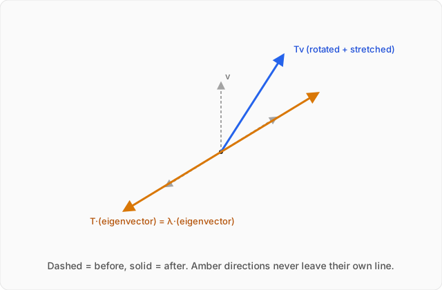
Linear Algebra: Eigenvalues, Eigenvectors, and Diagonalization

Take a vector and apply a typical linear operator. The result is usually longer or shorter, but it also points somewhere else. The operator has mixed two effects together: stretching and turning. After one application this may be manageable; after a hundred applications, the geometry can become nearly impossible to follow.

But perhaps the operator has a few privileged directions. Is there a nonzero vector that it does not turn at all? Along such a direction, the output would point exactly the same way as the input, or exactly opposite to it. The operator would do nothing there except multiply the vector by a number.

If we could find enough of those directions, the whole transformation would stop looking like a machine that mixes coordinates and start looking like several independent stretching machines. That is the idea behind eigenvectors, eigenvalues, and diagonalization. It is also why these objects appear whenever physics asks for repeated evolution, normal modes, stable axes, or possible measurement outcomes.

Eigenvalues and eigenvectors

Let $T$ be a linear operator on a vector space. A nonzero vector $\vec v$ is an eigenvector of $T$ if

T\vec v = \lambda \vec v

for some scalar $\lambda$ . The scalar $\lambda$ is the corresponding eigenvalue.

The requirement $\vec v\neq \vec 0$ matters. Since every linear operator sends $\vec 0$ to $\vec 0$ , allowing the zero vector would make it an uninformative eigenvector for every possible $\lambda$ .

The geometry is immediate. If $\lambda>0$ , the vector keeps its direction and changes length by a factor $|\lambda|$ . If $\lambda<0$ , it reverses direction and changes length by $|\lambda|$ . If $\lambda=0$ , the operator collapses that eigenvector to the zero vector. In every case, there is no sideways component: the operator does not rotate the eigenvector away from its own line.

This is the linear-algebra version of looking for a normal mode in a mechanical system. In a generic motion, several coordinates are mixed together. In a normal mode, the entire pattern reproduces itself under the dynamics, changing only by an overall factor or phase.

The characteristic equation

The definition tells us what an eigenvector does, but it does not yet tell us how to find one. Begin with

T\vec v=\lambda\vec v.

The scalar multiplication on the right can be written using the identity operator $I$ :

T\vec v=\lambda I\vec v.

Move everything to one side:

(T-\lambda I)\vec v=0.

For most values of $\lambda$ , the operator $T-\lambda I$ is invertible. If that were true here, multiplying both sides by $(T-\lambda I)^{-1}$ would force

\vec v=(T-\lambda I)^{-1}\vec 0=\vec 0,

which is forbidden. Therefore a nonzero solution can exist only when $T-\lambda I$ is singular. In a chosen basis, this becomes the determinant condition

\det(T-\lambda I)=0.

This is the characteristic equation. The expression

p_T(\lambda)=\det(T-\lambda I)

is the characteristic polynomial, and its roots are the eigenvalues of $T$ . For an $n\times n$ matrix, $p_T(\lambda)$ has degree $n$ , counting multiplicity.

Once an eigenvalue is known, substitute it back into

(T-\lambda I)\vec v=0

and solve for the nonzero vectors in the null space. Those vectors are the eigenvectors belonging to that eigenvalue.

A familiar spin calculation

The page on angular momentum and spin introduced the Pauli matrix

\sigma_z= \begin{pmatrix} 1 & 0\\ 0 & -1 \end{pmatrix}.

There, its special vectors and possible spin outcomes could be read off by inspection. Now apply the general method. Subtract $\lambda I$ :

\sigma_z-\lambda I= \begin{pmatrix} 1-\lambda & 0\\ 0 & -1-\lambda \end{pmatrix}.

The characteristic equation is

\det(\sigma_z-\lambda I) =(1-\lambda)(-1-\lambda)=0.

Equivalently,

\lambda^2-1=0,

\lambda=+1 \qquad\text{or}\qquad \lambda=-1.

For $\lambda=+1$ ,

(\sigma_z-I)\vec v= \begin{pmatrix} 0 & 0\\ 0 & -2 \end{pmatrix} \begin{pmatrix} v_1\\ v_2 \end{pmatrix} =\begin{pmatrix} 0\\ 0 \end{pmatrix},

which requires $v_2=0$ . One normalized eigenvector is

\vec v_+=\begin{pmatrix}1\\0\end{pmatrix}.

For $\lambda=-1$ ,

(\sigma_z+I)\vec v= \begin{pmatrix} 2 & 0\\ 0 & 0 \end{pmatrix} \begin{pmatrix} v_1\\ v_2 \end{pmatrix} =\begin{pmatrix} 0\\ 0 \end{pmatrix},

which requires $v_1=0$ . One normalized eigenvector is

\vec v_-=\begin{pmatrix}0\\1\end{pmatrix}.

This is the same computation already done on this site by inspection, now derived from the general method.

A 2D shear or stretch transformation shown acting on a grid of vectors, with the two special eigenvector directions highlighted where vectors only stretch or shrink without rotating, versus a generic vector which both rotates and stretches. — The operator turns a generic vector as it stretches it, but vectors lying along an eigenvector direction remain on their original line.

Diagonalization

Suppose an $n\times n$ matrix $T$ has $n$ linearly independent eigenvectors

\vec v_1,\vec v_2,\ldots,\vec v_n

with corresponding eigenvalues

\lambda_1,\lambda_2,\ldots,\lambda_n.

Because the eigenvectors are linearly independent, they form a basis. In that basis, the action of $T$ is especially transparent:

T\vec v_i=\lambda_i\vec v_i.

Each basis vector is sent only to a multiple of itself. Nothing is mixed into the other basis directions. Therefore the matrix of $T$ in the eigenvector basis is diagonal:

D= \begin{pmatrix} \lambda_1 & 0 & \cdots & 0\\ 0 & \lambda_2 & \cdots & 0\\ \vdots & \vdots & \ddots & \vdots\\ 0 & 0 & \cdots & \lambda_n \end{pmatrix}.

Let $P$ be the matrix whose columns are the eigenvectors:

P=\begin{pmatrix}\vec v_1 & \vec v_2 & \cdots & \vec v_n\end{pmatrix}.

Then

TP=PD,

because the $i$ th column on each side is $T\vec v_i=\lambda_i\vec v_i$ . Multiplying on the left by $P^{-1}$ gives

P^{-1}TP=D,

or equivalently,

T=PDP^{-1}.

This is diagonalization. It is not merely cosmetic. Consider applying $T$ one hundred times:

T^{100}=(PDP^{-1})^{100}.

Every neighboring pair $P^{-1}P$ cancels, leaving

T^{100}=PD^{100}P^{-1},

where

D^{100}= \begin{pmatrix} \lambda_1^{100} & 0 & \cdots & 0\\ 0 & \lambda_2^{100} & \cdots & 0\\ \vdots & \vdots & \ddots & \vdots\\ 0 & 0 & \cdots & \lambda_n^{100} \end{pmatrix}.

The same idea handles matrix exponentials, which appear throughout physics in time evolution and exponentials of Hamiltonians. Using the power-series definition,

e^T=I+T+\frac{T^2}{2!}+\frac{T^3}{3!}+\cdots,

and substituting $T=PDP^{-1}$ gives

e^T=Pe^DP^{-1},

with

e^D= \begin{pmatrix} e^{\lambda_1} & 0 & \cdots & 0\\ 0 & e^{\lambda_2} & \cdots & 0\\ \vdots & \vdots & \ddots & \vdots\\ 0 & 0 & \cdots & e^{\lambda_n} \end{pmatrix}.

A difficult coupled calculation has become $n$ independent scalar calculations. The only catch is important: not every matrix has $n$ linearly independent eigenvectors. A matrix is diagonalizable precisely when it has enough eigenvectors to form a basis.

Worked example

Find the eigenvalues and normalized eigenvectors of $A=\begin{pmatrix}2 & 1\\1 & 2\end{pmatrix}$ , then construct $P$ and verify that $P^{-1}AP$ is diagonal. (click to reveal the solution)

Setting up the characteristic equation: subtract $\lambda I$ from $A$ :

A-\lambda I= \begin{pmatrix} 2-\lambda & 1\\ 1 & 2-\lambda \end{pmatrix}.

A nonzero eigenvector exists only if this matrix is singular, so

\det(A-\lambda I)=0.

Expanding the determinant gives

(2-\lambda)(2-\lambda)-(1)(1)=0,

(2-\lambda)^2-1=0.

Expanding and factoring,

\lambda^2-4\lambda+3=0,

(\lambda-1)(\lambda-3)=0.

Therefore the eigenvalues are

\lambda_1=3, \qquad \lambda_2=1.

Eigenvector for $\lambda_1=3$ : solve

(A-3I)\vec v=0.

Writing $\vec v=\begin{pmatrix}x\\y\end{pmatrix}$ ,

\begin{pmatrix} -1 & 1\\ 1 & -1 \end{pmatrix} \begin{pmatrix} x\\y \end{pmatrix} = \begin{pmatrix} 0\\0 \end{pmatrix}.

The two rows give the same equation:

-x+y=0,

so $y=x$ . Every nonzero multiple of $\begin{pmatrix}1\\1\end{pmatrix}$ is an eigenvector. Its norm is

\left\|\begin{pmatrix}1\\1\end{pmatrix}\right\| =\sqrt{1^2+1^2}=\sqrt 2.

Thus a normalized eigenvector is

\vec u_1=\frac{1}{\sqrt 2} \begin{pmatrix} 1\\1 \end{pmatrix}.

Eigenvector for $\lambda_2=1$ : solve

(A-I)\vec v=0.

Then

\begin{pmatrix} 1 & 1\\ 1 & 1 \end{pmatrix} \begin{pmatrix} x\\y \end{pmatrix} = \begin{pmatrix} 0\\0 \end{pmatrix}.

Both rows give

x+y=0,

so $y=-x$ . Every nonzero multiple of $\begin{pmatrix}1\\-1\end{pmatrix}$ is an eigenvector. Its norm is

\left\|\begin{pmatrix}1\\-1\end{pmatrix}\right\| =\sqrt{1^2+(-1)^2}=\sqrt 2.

Thus a normalized eigenvector is

\vec u_2=\frac{1}{\sqrt 2} \begin{pmatrix} 1\\-1 \end{pmatrix}.

Constructing the change-of-basis matrix: place the normalized eigenvectors in columns, in the same order as their eigenvalues:

P= \begin{pmatrix} \vert & \vert\\ \vec u_1 & \vec u_2\\ \vert & \vert \end{pmatrix} = \frac{1}{\sqrt 2} \begin{pmatrix} 1 & 1\\ 1 & -1 \end{pmatrix}.

The columns are orthonormal, so $P$ is an orthogonal matrix and

P^{-1}=P^{\mathsf T}.

Here $P$ is also symmetric, so

P^{-1}=P^{\mathsf T}=P =\frac{1}{\sqrt 2} \begin{pmatrix} 1 & 1\\ 1 & -1 \end{pmatrix}.

Now calculate $AP$ first:

AP= \begin{pmatrix} 2 & 1\\ 1 & 2 \end{pmatrix} \frac{1}{\sqrt 2} \begin{pmatrix} 1 & 1\\ 1 & -1 \end{pmatrix} = \frac{1}{\sqrt 2} \begin{pmatrix} 3 & 1\\ 3 & -1 \end{pmatrix}.

Then

P^{-1}AP = \frac{1}{\sqrt 2} \begin{pmatrix} 1 & 1\\ 1 & -1 \end{pmatrix} \frac{1}{\sqrt 2} \begin{pmatrix} 3 & 1\\ 3 & -1 \end{pmatrix}.

Multiplying the matrices,

P^{-1}AP = \frac{1}{2} \begin{pmatrix} 6 & 0\\ 0 & 2 \end{pmatrix} = \begin{pmatrix} 3 & 0\\ 0 & 1 \end{pmatrix}.

The diagonal entries are exactly the eigenvalues, in the same order as the eigenvectors used as the columns of $P$ . In the original basis, $A$ mixes the two coordinates. In the eigenvector basis, it simply stretches the $\vec u_1$ direction by $3$ and leaves the $\vec u_2$ direction unchanged.

Where this leads

Eigenvalues are the mathematical machinery underneath measurement in quantum mechanics. The possible outcomes of measuring an observable are its eigenvalues, and the states left behind after measurement are its eigenvectors. That is precisely what the angular momentum and spin calculation did for spin before giving the procedure its general linear-algebra name.

The same method returns constantly. The eigenvectors of a coupled oscillator system are its normal modes. The eigenvectors of an inertia tensor identify the principal axes of rotation. Later in this track, vectors will give way to functions, matrices to differential operators, and eigenvectors to eigenfunctions, but the central question will remain unchanged: which states does the operator transform only by multiplication?