Linear Algebra: Vector Spaces and Linear Operators

Physics is crowded with things that can be added and scaled. Two displacements combine into a third displacement. Two electric fields superpose. Two possible quantum states can be added to form another state. Functions of time can be multiplied by numbers and added point by point. Even polynomials obey the same sort of arithmetic.

Only the first of these looks like the arrow introduced in kinematics. A polynomial has no obvious direction in physical space, and a quantum state is not a little arrow hidden inside an atom. Yet their algebra behaves so much like the algebra of arrows that using the same language is not a metaphor. It is a precise mathematical claim.

So what is the smallest set of rules that makes an object vector-like? Which properties actually mattered when we manipulated displacement, velocity, force, and fields, and which properties belonged only to the picture of an arrow with a length?

The answer is a vector space. Once we strip away the geometry and keep only the rules for addition and scaling, many apparently different physical objects become instances of one structure.

Vector spaces

A vector space $V$ over a field of scalars, usually $\mathbb{R}$ or $\mathbb{C}$ in physics, is a set equipped with two operations:

vector addition, which combines $\vec u,\vec v\in V$ to produce $\vec u+\vec v$ ;
scalar multiplication, which combines a scalar $a$ with $\vec v\in V$ to produce $a\vec v$ .

These operations must satisfy the following axioms for every $\vec u,\vec v,\vec w\in V$ and all scalars $a,b$ .

Closure under addition:
$\vec u+\vec v\in V.$
Associativity of addition:
$(\vec u+\vec v)+\vec w=\vec u+(\vec v+\vec w).$
Commutativity of addition:
$\vec u+\vec v=\vec v+\vec u.$
Existence of a zero vector: there is an element $\vec 0\in V$ such that
$\vec v+\vec 0=\vec v.$
Existence of additive inverses: for every $\vec v\in V$ , there is an element $-\vec v\in V$ such that
$\vec v+(-\vec v)=\vec 0.$
Closure under scalar multiplication:
$a\vec v\in V.$
Compatibility of scalar multiplication:
$a(b\vec v)=(ab)\vec v.$
Scalar identity:
$1\vec v=\vec v.$
Distributivity over vector addition:
$a(\vec u+\vec v)=a\vec u+a\vec v.$
Distributivity over scalar addition:
$(a+b)\vec v=a\vec v+b\vec v.$

These statements are deliberately abstract. They say nothing about arrows, angles, lengths, or coordinates. A vector space need not come with any notion of distance at all. It is the addition-and-scaling structure that earns its elements the name vectors.

Ordinary vectors in $\mathbb{R}^3$

The familiar example is

\mathbb{R}^3=\left\{ \begin{pmatrix} x\\y\\z \end{pmatrix}:x,y,z\in\mathbb{R} \right\}.

Addition and scalar multiplication are performed component by component:

\begin{pmatrix} x_1\\y_1\\z_1 \end{pmatrix} + \begin{pmatrix} x_2\\y_2\\z_2 \end{pmatrix} = \begin{pmatrix} x_1+x_2\\y_1+y_2\\z_1+z_2 \end{pmatrix},

and

a \begin{pmatrix} x\\y\\z \end{pmatrix} = \begin{pmatrix} ax\\ay\\az \end{pmatrix}.

The zero vector is $(0,0,0)$ , the additive inverse of $(x,y,z)$ is $(-x,-y,-z)$ , and the remaining axioms follow from the corresponding properties of real-number arithmetic. These are the displacement, velocity, acceleration, force, and electric-field vectors already used throughout mechanics and in Coulomb's law.

Quadratic polynomials as vectors

Now consider the set

P_2=\{ax^2+bx+c:a,b,c\in\mathbb{R}\},

the set of all real polynomials of degree at most two. Its elements are functions, not arrows. Nevertheless, define addition and scalar multiplication in the usual way. If

p(x)=a_1x^2+b_1x+c_1

and

q(x)=a_2x^2+b_2x+c_2,

then

p(x)+q(x) =(a_1+a_2)x^2+(b_1+b_2)x+(c_1+c_2).

The result is still a polynomial of degree at most two, so addition is closed. For a scalar $s$ ,

sp(x)=(sa_1)x^2+(sb_1)x+sc_1,

which is also in $P_2$ , so scalar multiplication is closed.

The zero vector in this space is the zero polynomial,

0x^2+0x+0,

and the additive inverse of $p(x)$ is

-p(x)=-a_1x^2-b_1x-c_1.

Associativity and commutativity follow because polynomial addition is coefficient-by-coefficient real-number addition. The distributive laws can be checked directly. For example,

s[p(x)+q(x)] =s[(a_1+a_2)x^2+(b_1+b_2)x+(c_1+c_2)]

becomes

(sa_1+sa_2)x^2+(sb_1+sb_2)x+(sc_1+sc_2),

which is exactly

sp(x)+sq(x).

Likewise,

(s+t)p(x)=sp(x)+tp(x),

s[tp(x)]=(st)p(x),

and

1p(x)=p(x).

Every vector-space axiom is present. The polynomial $2x^2-3x+1$ is therefore a vector in $P_2$ , just as $(2,-3,1)$ is a vector in $\mathbb{R}^3$ . In fact, the correspondence

2x^2-3x+1 \longleftrightarrow \begin{pmatrix} 2\\-3\\1 \end{pmatrix}

will soon turn out to be more than suggestive.

Linear combinations, independence, and basis

Given vectors $\vec v_1,\vec v_2,\ldots,\vec v_n$ , a linear combination is any vector of the form

a_1\vec v_1+a_2\vec v_2+\cdots+a_n\vec v_n.

The set of all such combinations is the span of those vectors. If their span equals the whole vector space $V$ , then they form a spanning set for $V$ .

But a spanning set can contain unnecessary vectors. In the plane, for example, three vectors may span every direction even though only two independent directions are needed. To identify redundancy, we ask whether the equation

a_1\vec v_1+a_2\vec v_2+\cdots+a_n\vec v_n=\vec 0

has any solution other than

a_1=a_2=\cdots=a_n=0.

If the trivial solution is the only solution, the vectors are linearly independent. If some coefficients are not zero, the vectors are linearly dependent, and at least one can be expressed as a linear combination of the others.

A basis of $V$ is a linearly independent set that spans $V$ . Equivalently, it is a minimal spanning set: remove any basis vector and the remaining vectors no longer span the whole space. Every vector in $V$ has one and only one expansion in a given basis.

The dimension of a finite-dimensional vector space is the number of vectors in any basis. Different bases may point in different directions or look like entirely different objects, but they all contain the same number of vectors.

The standard basis of $\mathbb{R}^3$ is

\hat x= \begin{pmatrix} 1\\0\\0 \end{pmatrix}, \qquad \hat y= \begin{pmatrix} 0\\1\\0 \end{pmatrix}, \qquad \hat z= \begin{pmatrix} 0\\0\\1 \end{pmatrix}.

Every ordinary vector can be written uniquely as

\vec v=v_x\hat x+v_y\hat y+v_z\hat z.

Mechanics has used this basis from the beginning, even when it was called only the $x$ , $y$ , and $z$ directions. Since it contains three vectors, $\mathbb{R}^3$ has dimension three.

The polynomial space $P_2$ has the basis

\{x^2,x,1\}.

Every $p(x)\in P_2$ can be written as

p(x)=ax^2+bx+c.

The three basis polynomials span $P_2$ , and they are linearly independent because

ax^2+bx+c=0

for every $x$ requires $a=b=c=0$ . Therefore

\dim P_2=3.

This is why a quadratic polynomial can be represented by the coordinate column

[p]_{\{x^2,x,1\}}= \begin{pmatrix} a\\b\\c \end{pmatrix}.

Coordinates do not belong to a vector by themselves. They describe a vector relative to a chosen basis.

Linear operators

A linear transformation is a map

T:V\to W

between vector spaces that respects linear combinations. For every $\vec u,\vec v\in V$ and all scalars $a,b$ ,

T(a\vec u+b\vec v)=aT(\vec u)+bT(\vec v).

When $V=W$ , the transformation is often called a linear operator on $V$ .

Linearity means that the transformation respects superposition. If two electric fields are added before an operation is performed, the result is the same as performing the operation on each field and then adding. This same structure lies behind the derivative operators used in vector calculus, since

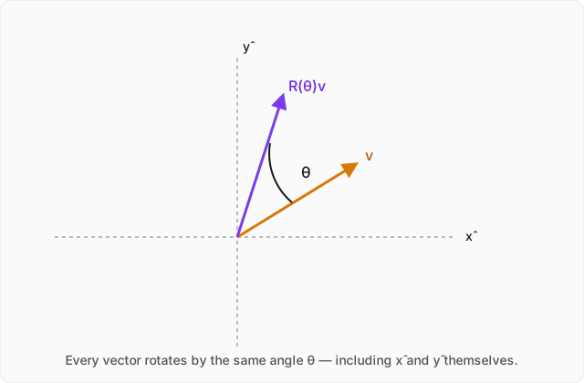
\frac{d}{dx}[af(x)+bg(x)] =a\frac{df}{dx}+b\frac{dg}{dx}.

A rotation of vectors in the plane is another linear operator. If two vectors are added and the sum is rotated, the result is the same as rotating each vector and then adding them. Scaling a vector before rotation is also the same as scaling it afterward.

Here is the crucial payoff: once bases have been chosen, every linear transformation between finite-dimensional vector spaces can be represented by a matrix. The columns of that matrix are the coordinates of the transformed basis vectors. Matrices are not a separate topic from vector spaces. They are linear operators after we have picked a basis.

To see why, let $\{\vec e_1,\ldots,\vec e_n\}$ be a basis of $V$ . Any vector can be written as

\vec v=v_1\vec e_1+\cdots+v_n\vec e_n.

By linearity,

T(\vec v) =v_1T(\vec e_1)+\cdots+v_nT(\vec e_n).

Once we know what $T$ does to every basis vector, we know what it does to every vector. Placing the coordinate vectors of $T(\vec e_1),\ldots,T(\vec e_n)$ into the columns of a matrix records the entire transformation.

Deriving the rotation matrix

Consider a counterclockwise rotation through an angle $\theta$ in the plane. Use the standard basis

\hat x= \begin{pmatrix} 1\\0 \end{pmatrix}, \qquad \hat y= \begin{pmatrix} 0\\1 \end{pmatrix}.

First track $\hat x$ . It begins at angle zero and ends at angle $\theta$ , so its rotated components are

R(\theta)\hat x= \begin{pmatrix} \cos\theta\\ \sin\theta \end{pmatrix}.

Now track $\hat y$ . It begins at angle $\pi/2$ and ends at angle $\pi/2+\theta$ . Therefore

R(\theta)\hat y= \begin{pmatrix} \cos(\pi/2+\theta)\\ \sin(\pi/2+\theta) \end{pmatrix}.

Using

\cos(\pi/2+\theta)=-\sin\theta

and

\sin(\pi/2+\theta)=\cos\theta,

we obtain

R(\theta)\hat y= \begin{pmatrix} -\sin\theta\\ \cos\theta \end{pmatrix}.

The images of the basis vectors become the columns of the matrix. Thus

R(\theta)= \begin{pmatrix} \cos\theta & -\sin\theta\\ \sin\theta & \cos\theta \end{pmatrix}.

Now take an arbitrary vector

\vec v= \begin{pmatrix} x\\y \end{pmatrix} =x\hat x+y\hat y.

Linearity gives

R(\theta)\vec v =xR(\theta)\hat x+yR(\theta)\hat y.

Substituting the rotated basis vectors,

R(\theta)\vec v =x \begin{pmatrix} \cos\theta\\ \sin\theta \end{pmatrix} +y \begin{pmatrix} -\sin\theta\\ \cos\theta \end{pmatrix}.

Combining components,

R(\theta)\vec v = \begin{pmatrix} x\cos\theta-y\sin\theta\\ x\sin\theta+y\cos\theta \end{pmatrix}.

This is exactly what ordinary matrix multiplication produces:

\begin{pmatrix} x'\\y' \end{pmatrix} = \begin{pmatrix} \cos\theta & -\sin\theta\\ \sin\theta & \cos\theta \end{pmatrix} \begin{pmatrix} x\\y \end{pmatrix} = \begin{pmatrix} x\cos\theta-y\sin\theta\\ x\sin\theta+y\cos\theta \end{pmatrix}.

The matrix is not an arbitrary rectangular array. Its first column says where $\hat x$ goes, its second column says where $\hat y$ goes, and linearity determines everything between them.

A 2D vector before and after being rotated by angle theta, showing the standard basis vectors x-hat and y-hat and where they map to under the rotation. — A rotation is fixed once the images of the two basis vectors are known; those two images become the columns of the rotation matrix.

Worked example

Verify directly that the rotation matrix $R(\theta)$ preserves the length of every vector $\vec v$ , and show explicitly that this follows from $R^{T}R=I$ . (click to reveal the solution)

Writing the rotation and its transpose: let

R= \begin{pmatrix} \cos\theta & -\sin\theta\\ \sin\theta & \cos\theta \end{pmatrix}.

Transposing exchanges rows and columns, so

R^T= \begin{pmatrix} \cos\theta & \sin\theta\\ -\sin\theta & \cos\theta \end{pmatrix}.

Multiplying $R^TR$ explicitly:

R^TR = \begin{pmatrix} \cos\theta & \sin\theta\\ -\sin\theta & \cos\theta \end{pmatrix} \begin{pmatrix} \cos\theta & -\sin\theta\\ \sin\theta & \cos\theta \end{pmatrix}.

Computing each entry gives

R^TR = \begin{pmatrix} \cos^2\theta+\sin^2\theta & -\cos\theta\sin\theta+\sin\theta\cos\theta \\ -\sin\theta\cos\theta+\cos\theta\sin\theta & \sin^2\theta+\cos^2\theta \end{pmatrix}.

The off-diagonal entries cancel, and the identity

\sin^2\theta+\cos^2\theta=1

reduces the product to

R^TR= \begin{pmatrix} 1&0\\ 0&1 \end{pmatrix} =I.

A real matrix satisfying $R^TR=I$ is called an orthogonal matrix. Equivalently,

R^{-1}=R^T.

For a rotation, this has a direct geometric meaning: rotating backward through $-\theta$ undoes rotating forward through $\theta$ .

Proving length preservation from orthogonality: the squared length of a column vector $\vec v$ is

|\vec v|^2=\vec v^{\,T}\vec v.

The rotated vector is $R\vec v$ , so its squared length is

|R\vec v|^2=(R\vec v)^T(R\vec v).

Using $(R\vec v)^T=\vec v^{\,T}R^T$ ,

|R\vec v|^2 =\vec v^{\,T}R^TR\vec v.

Since $R^TR=I$ ,

|R\vec v|^2 =\vec v^{\,T}I\vec v =\vec v^{\,T}\vec v =|\vec v|^2.

Lengths are nonnegative, so taking the square root gives

|R\vec v|=|\vec v|.

Checking the same result in components: for

\vec v= \begin{pmatrix} x\\y \end{pmatrix},

the rotated components are

x'=x\cos\theta-y\sin\theta

and

y'=x\sin\theta+y\cos\theta.

Therefore

|R\vec v|^2=(x')^2+(y')^2.

Substituting,

|R\vec v|^2 =(x\cos\theta-y\sin\theta)^2 +(x\sin\theta+y\cos\theta)^2.

Expanding both squares,

|R\vec v|^2 =x^2\cos^2\theta-2xy\sin\theta\cos\theta+y^2\sin^2\theta

\qquad +x^2\sin^2\theta+2xy\sin\theta\cos\theta+y^2\cos^2\theta.

The cross terms cancel. Grouping the remaining terms,

|R\vec v|^2 =x^2(\cos^2\theta+\sin^2\theta) +y^2(\sin^2\theta+\cos^2\theta).

Thus

|R\vec v|^2=x^2+y^2=|\vec v|^2,

and once again

|R\vec v|=|\vec v|.

The component calculation and the compact matrix calculation say the same thing. Orthogonality packages the length-preserving geometry of a rotation into the single equation $R^TR=I$ .

Where this leads

Vector spaces and linear operators are the language in which quantum mechanics is secretly written. Quantum states are vectors, though not generally arrows in ordinary space, and observables are linear operators acting on those states. On the page about angular momentum and spin, the eigenvalues and eigenvectors of Pauli matrices were already being computed without this general vocabulary.

The next topic makes that vocabulary explicit. An eigenvector is a special direction in a vector space along which a linear operator acts by pure scaling, with no turning into any other direction. Its scale factor is the corresponding eigenvalue. Finding those directions is what allows a complicated operator to reveal its simplest possible action.