Angular Momentum and Spin

Here is a classical picture you already know: set a wheel spinning, and its angular momentum can point in any direction and have any magnitude. In the language of rotational motion, $L = I\omega$ , torque changes angular momentum according to $\tau = dL/dt$ , and an isolated system conserves it. Nothing in Newtonian mechanics forces $L$ to come in steps.

Atoms refuse to cooperate with that picture. Their spectra show discrete patterns that make sense only if angular momentum is quantized. Nature does not permit an electron bound in an atom to carry just any orbital angular momentum or to point that angular momentum with just any projection along an axis.

Then comes the deeper surprise. An electron also carries angular momentum even when there is no orbital motion to blame. We call this intrinsic angular momentum spin, but the name is dangerous if taken too literally. The electron is not a tiny rigid ball rotating about an axis. Spin has no classical mechanical counterpart at all. It is a quantum property that behaves mathematically like angular momentum because it obeys the angular-momentum algebra.

Angular momentum becomes an operator

For orbital motion, the classical expression $\mathbf{L}=\mathbf{r}\times\mathbf{p}$ becomes the operator

\hat{\mathbf{L}}=\hat{\mathbf{r}}\times\hat{\mathbf{p}}.

In Cartesian components,

\hat{L}_x=\hat{y}\hat{p}_z-\hat{z}\hat{p}_y, \qquad \hat{L}_y=\hat{z}\hat{p}_x-\hat{x}\hat{p}_z, \qquad \hat{L}_z=\hat{x}\hat{p}_y-\hat{y}\hat{p}_x.

These look innocent until we calculate their commutators. Using the canonical relations $[\hat{x}_i,\hat{p}_j]=i\hbar\delta_{ij}$ , we find

[\hat{L}_x,\hat{L}_y]=i\hbar\hat{L}_z,

with the cyclic relations

[\hat{L}_y,\hat{L}_z]=i\hbar\hat{L}_x, \qquad [\hat{L}_z,\hat{L}_x]=i\hbar\hat{L}_y.

This non-commutativity is not a complaint about imperfect equipment. It says that no quantum state can assign simultaneously sharp values to all three components of angular momentum. If $L_x$ is definite, the state cannot in general also have definite $L_y$ and $L_z$ . The obstruction is built into the structure of the observables themselves.

For example, the uncertainty relation gives

\Delta L_x\,\Delta L_y \geq \frac{\hbar}{2}\left|\langle \hat{L}_z\rangle\right|.

So the quantum angular-momentum vector is not a classical arrow whose three coordinates merely happen to be hidden from us. The three components do not all possess sharp values at once.

What can be known together?

Although the components quarrel with one another, the total squared angular momentum

\hat{L}^2=\hat{L}_x^2+\hat{L}_y^2+\hat{L}_z^2

has a more peaceful relationship with every component. In particular,

[\hat{L}^2,\hat{L}_z]=0.

Therefore $\hat{L}^2$ and $\hat{L}_z$ can share simultaneous eigenstates. We label them $|l,m\rangle$ and define them by

\hat{L}^2|l,m\rangle=\hbar^2l(l+1)|l,m\rangle,

\hat{L}_z|l,m\rangle=\hbar m|l,m\rangle.

For orbital angular momentum,

l=0,1,2,\ldots, \qquad m=-l,-l+1,\ldots,l-1,l.

A state with quantum number $l$ therefore has a fixed angular-momentum magnitude

|\mathbf{L}|=\sqrt{l(l+1)}\,\hbar,

but only a definite projection along the chosen $z$ -axis,

L_z=m\hbar.

Notice the small but important geometric shock: even in the state with the largest possible projection, $m=l$ , the magnitude is $\sqrt{l(l+1)}\hbar$ , which is larger than $l\hbar$ . The angular momentum is never completely aligned with the $z$ -axis in the classical sense. The transverse components cannot both vanish sharply.

The ladder appears again

This spectrum is not guessed. It follows from exactly the same algebraic strategy used for the quantum harmonic oscillator. Recall the pattern from that topic:

Define two new operators: $\hat{a} = \sqrt{m\omega/2\hbar}(\hat{x} + i\hat{p}/m\omega)$ , $\hat{a}^{\dagger} = \sqrt{m\omega/2\hbar}(\hat{x} - i\hat{p}/m\omega)$ . Their commutator is $[\hat{a},\hat{a}^{\dagger}] = 1$ . The Hamiltonian becomes $\hat{H} = \hbar\omega(\hat{a}^{\dagger}\hat{a} + 1/2)$ . Define the number operator $\hat{N} = \hat{a}^{\dagger}\hat{a}$ . Using only $[\hat{a},\hat{a}^{\dagger}]=1$ , one shows $\hat{a}^{\dagger}|n\rangle = \sqrt{n+1}|n+1\rangle$ (raises $n$ by one) and $\hat{a}|n\rangle = \sqrt{n}|n-1\rangle$ (lowers $n$ by one). Since $\hat{a}$ can't lower forever without hitting negative probabilities, there must be a ground state $|0\rangle$ with $\hat{a}|0\rangle = 0$ , and the whole ladder of states is built by repeatedly applying $\hat{a}^{\dagger}$ to $|0\rangle$ . This gave $E_n = \hbar\omega(n + 1/2)$ .

Now make the angular-momentum combinations

\hat{L}_{\pm}=\hat{L}_x\pm i\hat{L}_y.

This is the same mathematical trick as $\hat{a}$ and $\hat{a}^{\dagger}$ : define a raising/lowering combination, build a ladder, and find where it terminates. The relevant commutators are

[\hat{L}_z,\hat{L}_{\pm}]=\pm\hbar\hat{L}_{\pm}, \qquad [\hat{L}^2,\hat{L}_{\pm}]=0.

Therefore $\hat{L}_{\pm}$ changes $m$ without changing $l$ :

\hat{L}_{\pm}|l,m\rangle = \hbar\sqrt{l(l+1)-m(m\pm1)}\,|l,m\pm1\rangle.

The ladder cannot rise or fall forever. Its upper and lower ends occur at

m_{\max}=l, \qquad m_{\min}=-l,

where

\hat{L}_+|l,l\rangle=0, \qquad \hat{L}_-|l,-l\rangle=0.

So a fixed $l$ gives exactly $2l+1$ allowed values of $m$ . The oscillator ladder is infinite above and stops only at the bottom. The angular-momentum ladder stops at both ends. Different physical problem, same algebraic instinct.

Spin: angular momentum without orbital motion

Some particles possess an additional angular momentum $\hat{\mathbf{S}}$ . It obeys the same commutation algebra,

[\hat{S}_x,\hat{S}_y]=i\hbar\hat{S}_z,

and cyclic permutations, but it is not constructed from $\hat{\mathbf{r}}\times\hat{\mathbf{p}}$ . It is intrinsic. Asking what material inside the electron is rotating is therefore the wrong question, rather like asking which little gears inside a photon make it travel at the speed of light.

Spin states are labeled $|s,m_s\rangle$ :

\hat{S}^2|s,m_s\rangle = \hbar^2s(s+1)|s,m_s\rangle,

\hat{S}_z|s,m_s\rangle = \hbar m_s|s,m_s\rangle.

For a spin- $1/2$ particle such as the electron,

s=\frac{1}{2}, \qquad m_s=+\frac{1}{2}\ \text{or}\ -\frac{1}{2}.

That is the whole ladder: two states. Relative to a chosen axis, an electron can yield only spin up or spin down. Its total spin magnitude is fixed:

|\mathbf{S}|=\sqrt{s(s+1)}\,\hbar=\frac{\sqrt{3}}{2}\hbar.

Again, neither allowed $z$ -projection, $\pm\hbar/2$ , equals the full magnitude. Spin is not a tiny arrow secretly pointing exactly up or down. The two outcomes describe what happens when one component is measured.

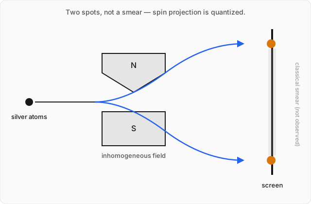
The Stern-Gerlach experiment: a beam of silver atoms passing through an inhomogeneous magnetic field splits into exactly two discrete beams rather than a continuous spread. — An inhomogeneous magnetic field turns angular-momentum projection into a visible deflection. Instead of painting a continuous stripe, the silver-atom beam separates into two distinct traces, revealing two allowed spin projections along the measurement axis.

The Stern-Gerlach apparatus makes the discreteness almost embarrassingly concrete. If the relevant magnetic moments had arbitrary orientations, the atoms would spread continuously across the detector. They do not. The beam splits. For the effective spin- $1/2$ degree of freedom, the apparatus returns one of two outcomes.

Worked example

Using the $2\times2$ Pauli-matrix representation, find the eigenvalues and normalized eigenvectors of $\hat{S}_z=(\hbar/2)\sigma_z$ . (click to reveal the solution)

Setting up: In the standard basis, the Pauli matrix $\sigma_z$ is

\sigma_z= \begin{pmatrix} 1 & 0\\ 0 & -1 \end{pmatrix}.

Therefore

\hat{S}_z=\frac{\hbar}{2}\sigma_z = \begin{pmatrix} \hbar/2 & 0\\ 0 & -\hbar/2 \end{pmatrix}.

We seek nonzero column vectors $\chi$ satisfying

\hat{S}_z\chi=\lambda\chi.

The eigenvalues follow from the characteristic equation

\det(\hat{S}_z-\lambda I)=0.

Substituting the matrix gives

\det \begin{pmatrix} \hbar/2-\lambda & 0\\ 0 & -\hbar/2-\lambda \end{pmatrix} =0,

\left(\frac{\hbar}{2}-\lambda\right) \left(-\frac{\hbar}{2}-\lambda\right)=0.

Hence the two eigenvalues are

\lambda_+=+\frac{\hbar}{2}, \qquad \lambda_-=-\frac{\hbar}{2}.

Eigenvector for $+\hbar/2$ : Let

\chi_+= \begin{pmatrix} a\\b \end{pmatrix}.

Then

\left(\hat{S}_z-\frac{\hbar}{2}I\right)\chi_+ = \begin{pmatrix} 0 & 0\\ 0 & -\hbar \end{pmatrix} \begin{pmatrix} a\\b \end{pmatrix} =0.

This requires $b=0$ , while $a$ is arbitrary and nonzero. Choosing unit norm gives

\chi_+= \begin{pmatrix} 1\\0 \end{pmatrix} \equiv |{+z}\rangle.

Indeed,

\hat{S}_z \begin{pmatrix} 1\\0 \end{pmatrix} = \frac{\hbar}{2} \begin{pmatrix} 1\\0 \end{pmatrix}.

This is the familiar spin-up state along $z$ .

Eigenvector for $-\hbar/2$ : Write

\chi_-= \begin{pmatrix} a\\b \end{pmatrix}.

Now

\left(\hat{S}_z+\frac{\hbar}{2}I\right)\chi_- = \begin{pmatrix} \hbar & 0\\ 0 & 0 \end{pmatrix} \begin{pmatrix} a\\b \end{pmatrix} =0.

This requires $a=0$ . Choosing unit norm gives

\chi_-= \begin{pmatrix} 0\\1 \end{pmatrix} \equiv |{-z}\rangle.

Indeed,

\hat{S}_z \begin{pmatrix} 0\\1 \end{pmatrix} = -\frac{\hbar}{2} \begin{pmatrix} 0\\1 \end{pmatrix}.

This is the familiar spin-down state along $z$ .

Result: The matrix $\hat{S}_z$ has exactly the two allowed measurement outcomes

S_z=+\frac{\hbar}{2} \quad\text{and}\quad S_z=-\frac{\hbar}{2},

with normalized eigenvectors

|{+z}\rangle= \begin{pmatrix} 1\\0 \end{pmatrix}, \qquad |{-z}\rangle= \begin{pmatrix} 0\\1 \end{pmatrix}.

A general normalized spin state can be a superposition $\alpha|{+z}\rangle+\beta|{-z}\rangle$ , with $|\alpha|^2+|\beta|^2=1$ , but a measurement of $S_z$ still returns only one of these two eigenvalues.

Where this leads

Angular momentum and spin complete the core toolkit of non-relativistic quantum mechanics, right where the quantum track meets rotational motion. From here, the track continues toward special relativity on a separate branch and eventually toward quantum field theory, where spin is not merely another quantum number: it determines whether a particle is a fermion or a boson.