The Maxwell-Boltzmann Distribution

The previous topic ended with a clean, satisfying equation: $\frac{1}{2}m\langle v^2\rangle = \frac{3}{2}k_BT$. It's tempting to read that as "every molecule in the gas moves at speed $\sqrt{3k_BT/m}$." That reading is wrong, and it's worth being precise about why.

$\langle v^2 \rangle$ is an average — computed over an enormous number of molecules that are constantly colliding with each other, trading energy back and forth in every encounter. Right after a collision, one molecule might be launched at three times its old speed while the one it hit nearly stops. A moment later, a different pair does the same thing in reverse. There is no mechanism in this picture that could make every molecule settle on one common speed — quite the opposite: collisions are exactly what keeps scrambling the individual speeds, second by second, molecule by molecule. What stays fixed, even while every individual molecule's speed is churning, is the overall statistical pattern of speeds across the whole population. That pattern is what this topic finds, exactly.

This is precisely the kind of question probability and statistics was built to answer: not "what is the one value of $v$," but "what is the probability distribution over all possible values of $v$" — a continuous distribution, since speed isn't restricted to a discrete list of allowed values the way, say, a coin flip is.

Two physical assumptions, and the algebra they force

Here is Maxwell's own argument, and it is worth following closely because it derives the distribution's shape from almost nothing.

Work first with the velocity components $(v_x,v_y,v_z)$ rather than the speed itself, and make two physical assumptions about the probability density $f(v_x,v_y,v_z)$ for a molecule to have a given velocity:

1. Independence. The three components are statistically independent of one another — knowing $v_x$ tells you nothing about $v_y$. This lets the joint density factor: $f(v_x,v_y,v_z) = g(v_x)\,g(v_y)\,g(v_z)$, for some single-variable function $g$ that is the same for all three directions (nothing in an ordinary gas picks out $x$, $y$, or $z$ as special).
2. Isotropy. The gas has no preferred direction at all, so the density can only depend on the speed, not the direction of travel: $f(v_x,v_y,v_z) = F(v_x^2+v_y^2+v_z^2)$ for some function $F$.

Put those together:

Take the logarithm of both sides, and define $h \equiv \ln g$ and $H \equiv \ln F$:

Differentiate with respect to $v_x$, holding $v_y,v_z$ fixed (the chain rule picks up a factor of $2v_x$ on the right):

Do the same with respect to $v_y$:

Divide one by the other, and $H'$ — the same function, evaluated at the same argument in both equations — cancels completely:

The left side depends only on $v_x$; the right side only on $v_y$. Since $v_x$ and $v_y$ can be varied completely independently of one another, the only way this equation can hold for every choice of both is if each side is the same constant, call it $2a$:

Exponentiating back, $g(v_x) = Ce^{av_x^2}$. For this to be a normalizable probability density (one that doesn't blow up as $v_x\to\pm\infty$), $a$ must be negative — write $a = -1/(2\sigma^2)$. Isotropy and independence, together, have forced the distribution of each velocity component to be a Gaussian — precisely the bell-shaped curve that appears throughout probability and statistics as the limit the central limit theorem points to, though here it arrives by a completely different, purely mechanical route.

Fixing the width with what we already know

The one thing left undetermined is $\sigma^2$, and the previous topic already handed us the answer. We found $\frac{1}{2}m\langle v^2\rangle = \frac32k_BT$, and by the same isotropy used there, $\langle v_x^2\rangle = \frac13\langle v^2\rangle = \frac{k_BT}{m}$. A Gaussian $g(v_x)\propto e^{-v_x^2/2\sigma^2}$ has variance exactly $\sigma^2 = \langle v_x^2\rangle$, so $\sigma^2 = k_BT/m$. Normalizing $g$ to integrate to $1$ (the standard Gaussian integral $\int e^{-ax^2}dx=\sqrt{\pi/a}$) gives the fully specified single-component distribution:

From velocity components to speed

We want the distribution of speed $v = \sqrt{v_x^2+v_y^2+v_z^2}$, not of any one component. Multiply the three component distributions together to get the full joint density in velocity space:

This depends only on $v$, exactly as isotropy demanded — it assigns equal probability density to every direction at a fixed speed. To find the probability of the speed itself falling in a small range $[v,v+dv]$, we need to add up this density over every direction consistent with that speed: a thin spherical shell in velocity space, of radius $v$ and thickness $dv$, whose volume is $4\pi v^2\,dv$ (the same geometric fact that gives a sphere's surface area). Multiplying the density by that shell volume gives the Maxwell-Boltzmann speed distribution:

Two competing effects are visible directly in this formula, and their tug-of-war is the whole story of its shape: the $v^2$ factor grows with speed (there's simply more "room" — more directions — at larger speeds), while the exponential falls off (fast molecules are exponentially rarer). The result is a curve that starts at zero, rises to a single peak, and decays back toward zero — never symmetric, always with a longer tail toward high speeds than toward low ones.

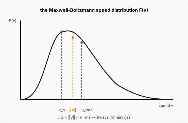
Three different "typical" speeds

Because the curve isn't symmetric, "the typical speed" splits into (at least) three legitimately different numbers, each answering a different question.

Most probable speed $v_p$: where the curve peaks. Set $dF/dv=0$. Since $F(v)\propto v^2e^{-mv^2/2k_BT}$, product rule gives $\frac{d}{dv}\left(v^2e^{-mv^2/2k_BT}\right) = e^{-mv^2/2k_BT}\left(2v - \frac{mv^3}{k_BT}\right)$, which vanishes (for $v\neq0$) when $2 = mv^2/k_BT$:

Mean speed $\langle v\rangle$: the expectation value of $v$ under this distribution, exactly the integral construction from probability and statistics applied to a continuous variable, $\langle v\rangle = \int_0^\infty v\,F(v)\,dv$. Carrying out that integral (it requires one integration by parts and the same family of Gaussian integrals used above) gives:

Root-mean-square speed $v_{\text{rms}} = \sqrt{\langle v^2\rangle}$: this is the one we already know, straight from the previous topic's $\frac12m\langle v^2\rangle = \frac32 k_BT$:

Compare the numerical coefficients inside the square roots: $2 < 8/\pi\approx2.55 < 3$. So $v_p < \langle v\rangle < v_{\text{rms}}$, always, for any gas at any temperature — a direct fingerprint of the distribution's asymmetry, since a symmetric distribution would force all three to coincide.

Worked example

Where this leads

We now have the exact statistical shape of molecular speeds in an ordinary gas at equilibrium — but notice what we still don't have an explanation for. Why a Gaussian, mechanically? Isotropy and independence forced the functional form, but nothing here explained why a system left alone settles into this particular distribution and stays there, rather than some other distribution, or none at all. Answering that question properly requires stepping back from gases specifically and asking a much more general question: given a huge number of possible configurations a system could be in, why do some configurations dominate overwhelmingly over others? That is the question the next topic takes up from scratch, and it is the deepest idea in this entire track.