Probability and Statistics

Go back to the moment quantum mechanics first asked you to trust something new: the Born rule,

\rho(x,t) = |\psi(x,t)|^2,

introduced there as the probability density for finding a particle at position $x$ . Everything that followed on that page — normalization, the probability of finding a particle between two points, the entire physical meaning of the wave function — leaned on the word "probability" as though its meaning were already settled. It never was, formally. You were handed a working intuition and asked to run with it, which is a perfectly reasonable thing to do in a physics course, but it leaves a debt outstanding. This topic pays it: what a probability distribution actually is, how to extract a single representative number (the expectation value) and a measure of spread (the variance) from one, and why an enormous range of unrelated random processes — coin flips, molecular velocities, measurement errors, populations of anything — all funnel toward the exact same bell-shaped curve in the end.

Discrete probability distributions

A discrete random variable $X$ takes one of a finite (or countably infinite) list of values $x_1,x_2,\ldots$ , each with an associated probability $P(X=x_i)$ , often abbreviated $p_i$ . Two conditions make this bookkeeping consistent with the plain meaning of "probability":

0\leq p_i\leq1\quad\text{for every }i, \qquad \sum_i p_i = 1.

The second condition says the outcomes are exhaustive: something in the list is guaranteed to happen. This is the discrete cousin of the normalization condition $\int|\psi|^2dx=1$ already met for the wave function — the same statement, "the total probability of all possibilities is $1$ ," written as a sum instead of an integral because the outcomes here are a discrete list rather than a continuum of positions.

Continuous probability distributions

When the random variable can take any value in a continuous range — a position, a speed, a measurement error — a single number $p_i$ per outcome stops making sense, since there are uncountably many outcomes and each individual one typically has probability exactly zero. What survives is a probability density $\rho(x)$ , defined so that the probability of landing in a small interval is

P(a\leq X\leq b) = \int_a^b\rho(x)\,dx,

with normalization

\int_{-\infty}^{\infty}\rho(x)\,dx = 1.

This is exactly the structure the Born rule already used, with $\rho(x)=|\psi(x)|^2$ as one particular, physically singled-out choice of density. Nothing about the mathematics of $\rho$ required it to come from a wave function; a probability density is a general object, and $|\psi|^2$ is one instance of it, arriving with an unusually strange physical origin story but obeying completely ordinary rules once it exists.

Expectation value and variance

Given a distribution, the single most useful summary number is the expectation value (or mean), the probability-weighted average of the random variable. For a discrete distribution,

\langle X\rangle = \sum_i x_ip_i,

and for a continuous one,

\langle X\rangle = \int_{-\infty}^{\infty}x\,\rho(x)\,dx.

More generally, the expectation value of any function $f(X)$ of the random variable is defined the same way, weighting each value of $f$ by the probability of the underlying outcome:

\langle f(X)\rangle = \sum_i f(x_i)p_i \qquad\text{or}\qquad \langle f(X)\rangle = \int_{-\infty}^{\infty}f(x)\,\rho(x)\,dx.

The mean says where a distribution is centered, but says nothing about how tightly it's clustered around that center. That is the job of the variance,

\operatorname{Var}(X) = \left\langle(X-\langle X\rangle)^2\right\rangle,

the average squared deviation from the mean. Expanding the square and using linearity of the expectation value,

\operatorname{Var}(X) = \langle X^2 - 2X\langle X\rangle + \langle X\rangle^2\rangle = \langle X^2\rangle - 2\langle X\rangle\langle X\rangle + \langle X\rangle^2 = \langle X^2\rangle - \langle X\rangle^2,

using that $\langle X\rangle$ is just a constant number that can be pulled outside its own expectation value. This is the standard working formula for variance: mean of the square, minus square of the mean. Its square root, $\sigma=\sqrt{\operatorname{Var}(X)}$ , is the standard deviation, carrying the same units as $X$ itself and serving as the natural measure of how spread out the distribution is.

The binomial distribution

Consider $n$ independent trials, each succeeding with probability $p$ and failing with probability $1-p$ — flipping a coin, say, or checking whether each of $n$ radioactive nuclei has decayed in some fixed time window. Let $X$ be the total number of successes. The probability of getting exactly $k$ successes is

P(X=k) = \binom{n}{k}p^k(1-p)^{n-k}, \qquad \binom{n}{k}=\frac{n!}{k!(n-k)!},

the binomial distribution. The binomial coefficient counts the number of distinct orderings of $k$ successes and $n-k$ failures among $n$ trials, and each such ordering has probability $p^k(1-p)^{n-k}$ by independence, so their sum over all $\binom{n}{k}$ orderings gives the formula above.

Rather than grinding that sum out directly against the binomial formula, there's a shortcut: write $X$ as a sum of $n$ single trials, $X = X_1 + X_2 + \cdots + X_n$ , where each $X_i$ is a Bernoulli variable — it equals $1$ if trial $i$ succeeds and $0$ if it fails. A single trial's mean is easy:

\langle X_i\rangle = 1\cdot p + 0\cdot(1-p) = p.

For the variance, note that $X_i$ only ever takes the values $0$ and $1$ , and both of those satisfy $X_i^2=X_i$ — squaring a bit doesn't change it. So $\langle X_i^2\rangle=\langle X_i\rangle=p$ , and the working formula for variance derived above gives

\operatorname{Var}(X_i) = \langle X_i^2\rangle - \langle X_i\rangle^2 = p - p^2 = p(1-p).

Now extend to all $n$ trials. Expectation is linear no matter what — independent or not — so the mean of the sum is just the sum of the means:

\langle X\rangle = \langle X_1\rangle+\cdots+\langle X_n\rangle = np.

Variance doesn't add so freely in general: $\operatorname{Var}(X_1+X_2)=\operatorname{Var}(X_1)+\operatorname{Var}(X_2)+2\operatorname{Cov}(X_1,X_2)$ , and that cross term only vanishes when the trials don't influence each other. That's exactly what independence buys here — $\operatorname{Cov}(X_i,X_j)=\langle X_iX_j\rangle-\langle X_i\rangle\langle X_j\rangle=0$ for $i\neq j$ , since $\langle X_iX_j\rangle$ factors into $\langle X_i\rangle\langle X_j\rangle$ when the two trials are independent. All the cross terms drop out, leaving

\langle X\rangle = np, \qquad \operatorname{Var}(X) = np(1-p).

The Gaussian distribution as a limit

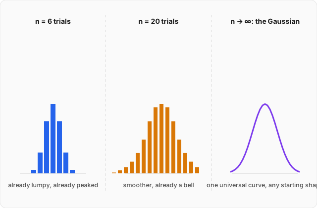
Here is the remarkable fact this topic is building toward. Take the binomial distribution and let $n$ grow very large while $p$ stays fixed. The distribution's shape, plotted as a function of $k$ , becomes smoother and smoother, and in the limit $n\to\infty$ it approaches a specific continuous curve — the Gaussian, or normal distribution,

\rho(x) = \frac{1}{\sigma\sqrt{2\pi}}\,e^{-(x-\mu)^2/2\sigma^2},

with $\mu=\langle X\rangle$ and $\sigma^2=\operatorname{Var}(X)$ matching the mean and variance of the distribution it's approximating. This is not a special property of coin flips. The central limit theorem states, in far greater generality, that the sum (or average) of a large number of independent random variables — drawn from any distribution with finite mean and variance, not only a binomial one — approaches a Gaussian distribution as the number of terms grows, regardless of the shape of the original distribution being summed. The theorem is not proven here in full generality, but the binomial-to-Gaussian limit worked below is its cleanest concrete instance: a distribution built from a sharply discrete, lopsided-looking process (a coin that might not even be fair) smooths itself into the single universal bell shape as more and more trials are piled on.

This is why the Gaussian shows up constantly and everywhere in physics: measurement noise, the velocities of molecules in a gas, the diffusion of a dye through water — anything that is itself the accumulated result of many small, roughly independent random contributions ends up looking Gaussian, almost regardless of the messy details of any one contribution.

Three panels showing a discrete binomial distribution for a small number of trials as blue bars, the same binomial distribution for a much larger number of trials as amber bars now visibly bell-shaped, and a smooth continuous Gaussian curve in purple overlaid on the same axis. — As the number of binomial trials grows, the discrete distribution of outcomes smooths into the continuous Gaussian curve — the central limit theorem, seen in one concrete case.

Worked example

A discrete random variable $X$ takes the values $1,2,3$ with probabilities $0.2,\ 0.5,\ 0.3$ respectively. Compute $\langle X\rangle$ and $\operatorname{Var}(X)$ . Then, for the normalized Gaussian $\rho(x)=\frac{1}{\sigma\sqrt{2\pi}}e^{-(x-\mu)^2/2\sigma^2}$ , verify by direct integration that $\langle X\rangle=\mu$ and that the standard deviation really is $\sigma$ . (click to reveal the solution)

The discrete case — computing the mean: by definition,

\langle X\rangle = \sum_i x_ip_i = (1)(0.2) + (2)(0.5) + (3)(0.3) = 0.2+1.0+0.9 = 2.0.

Computing $\langle X^2\rangle$ :

\langle X^2\rangle = \sum_i x_i^2p_i = (1)^2(0.2) + (2)^2(0.5) + (3)^2(0.3) = 0.2+2.0+2.7 = 4.9.

Computing the variance:

\operatorname{Var}(X) = \langle X^2\rangle - \langle X\rangle^2 = 4.9 - (2.0)^2 = 4.9-4.0 = 0.9.

So this distribution has mean $2.0$ and standard deviation $\sigma=\sqrt{0.9}\approx0.949$ .

The Gaussian case — setting up: the claim to check is

\int_{-\infty}^{\infty}x\,\rho(x)\,dx=\mu, \qquad \int_{-\infty}^{\infty}(x-\mu)^2\rho(x)\,dx=\sigma^2,

given that $\rho(x)$ is already normalized, $\int_{-\infty}^{\infty}\rho(x)\,dx=1$ (which follows from the standard Gaussian integral $\int_{-\infty}^{\infty}e^{-u^2/2\sigma^2}du=\sigma\sqrt{2\pi}$ , taken as known here). Substitute $u=x-\mu$ throughout, so $x=u+\mu$ and $dx=du$ , with $u$ ranging over the same $(-\infty,\infty)$ :

\langle X\rangle = \frac{1}{\sigma\sqrt{2\pi}}\int_{-\infty}^{\infty}(u+\mu)\,e^{-u^2/2\sigma^2}\,du = \frac{1}{\sigma\sqrt{2\pi}}\int_{-\infty}^{\infty}u\,e^{-u^2/2\sigma^2}\,du + \mu\cdot\frac{1}{\sigma\sqrt{2\pi}}\int_{-\infty}^{\infty}e^{-u^2/2\sigma^2}\,du.

Evaluating the first piece: the integrand $u\,e^{-u^2/2\sigma^2}$ is an odd function of $u$ (odd times even), and the integral of an odd function over the symmetric interval $(-\infty,\infty)$ vanishes — the same argument already used repeatedly on this site for odd integrands on symmetric intervals:

\int_{-\infty}^{\infty}u\,e^{-u^2/2\sigma^2}\,du = 0.

Evaluating the second piece: the remaining integral is exactly the normalization integral, equal to $\sigma\sqrt{2\pi}$ by assumption, so

\mu\cdot\frac{1}{\sigma\sqrt{2\pi}}\cdot\sigma\sqrt{2\pi} = \mu.

Adding both pieces,

\langle X\rangle = 0 + \mu = \mu,

confirming that the parameter $\mu$ appearing in the Gaussian formula really is its mean.

Checking the variance: with the same substitution $u=x-\mu$ ,

\operatorname{Var}(X) = \frac{1}{\sigma\sqrt{2\pi}}\int_{-\infty}^{\infty}u^2\,e^{-u^2/2\sigma^2}\,du.

This integral is evaluated by differentiating the normalization integral with respect to a parameter — a standard trick. Write $I(a)=\int_{-\infty}^{\infty}e^{-au^2}\,du=\sqrt{\pi/a}$ (the Gaussian integral, with $a=1/2\sigma^2$ here). Differentiating both sides with respect to $a$ :

\frac{dI}{da} = \int_{-\infty}^{\infty}(-u^2)\,e^{-au^2}\,du = -\frac{1}{2}\sqrt{\pi}\,a^{-3/2}.

\int_{-\infty}^{\infty}u^2e^{-au^2}\,du = \frac{\sqrt\pi}{2}a^{-3/2}.

Substituting $a=1/2\sigma^2$ , so $a^{-3/2}=(2\sigma^2)^{3/2}$ :

\int_{-\infty}^{\infty}u^2e^{-u^2/2\sigma^2}\,du = \frac{\sqrt\pi}{2}(2\sigma^2)^{3/2} = \frac{\sqrt\pi}{2}\cdot2\sqrt2\,\sigma^3 = \sqrt{2\pi}\,\sigma^3.

Dividing by the normalization factor $\sigma\sqrt{2\pi}$ :

\operatorname{Var}(X) = \frac{1}{\sigma\sqrt{2\pi}}\cdot\sqrt{2\pi}\,\sigma^3 = \sigma^2.

So the variance really is $\sigma^2$ , and the standard deviation of the Gaussian is exactly the parameter $\sigma$ appearing in its own formula — confirming that the two letters $\mu$ and $\sigma$ written into the Gaussian at the start of this topic were not arbitrary labels. They are, respectively, exactly the mean and exactly the standard deviation, verified here by direct integration rather than assumed.

Where this leads

Probability has now been built as a formal structure in its own right, with the Gaussian identified as the shape a huge class of accumulated random processes converges toward. That convergence is not a mathematical curiosity waiting for an application — it is the entire foundation of statistical mechanics, where the enormous number of particles in even a small gas sample means the accumulated randomness of countless individual collisions settles, via exactly this central-limit mechanism, into sharp, reliable, macroscopic laws. The next stretch of this site takes that idea and runs with it directly: the kinetic theory of gases derives the pressure and temperature of a gas from the statistics of its molecules' motion, and the distribution of molecular speeds is a direct descendant of the expectation-value and variance machinery built here. Beyond that, microstates and entropy shows that the number of ways a system's constituents can be arranged is itself the concept underlying temperature and the arrow of time — probability, in the end, is the machinery beneath the Second Law.