Imagine a storm damages a major port just as households are cutting back on spending. One force makes it harder for firms to produce; the other means buyers want less. If output falls and prices rise, which force did it? If output falls and inflation eases, what changed? We need a model with both sides of the economy in view.
The aggregate-demand and aggregate-supply model—AD–AS—places the overall price level and real output together. It is not a literal photograph of an economy. It is a map for asking how spending, production costs, and productive capacity can interact, and for seeing why different shocks need not have the same consequences.
The two axes
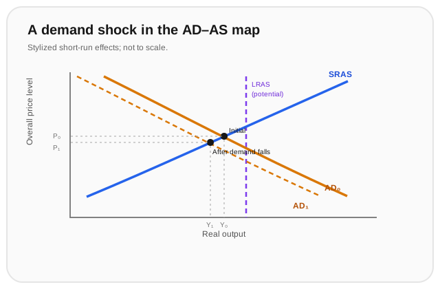
The horizontal axis measures real output, usually real GDP. The vertical axis measures the economy-wide price level. Aggregate demand (AD) describes planned purchases of domestic output at different price levels. Aggregate supply describes how much firms are willing and able to produce at different price levels under specified conditions.
The intersection of AD and short-run aggregate supply (SRAS) gives a short-run equilibrium in the model. “Equilibrium” here means the curves intersect; it does not mean everyone has a job, firms are perfectly satisfied, or the outcome is fair. The model gives us a starting point for tracking changes.
Why aggregate demand slopes downward
The downward slope of AD does not mean that every household buys more of every good whenever prices fall. It summarizes several economy-wide channels. If the overall price level falls while nominal incomes and money balances are temporarily unchanged, existing balances buy more. Interest rates and borrowing conditions may change, affecting investment and durable purchases. Relative prices can also alter imports and exports. These mechanisms are simplified in the introductory model; their strength depends on institutions and circumstances.
Changes in confidence, government purchases, taxes, expected future income, financing conditions, or foreign demand can shift AD. A change in the overall price level is instead represented as movement along a given AD curve, when the other influences are held fixed.
Short-run supply and long-run capacity
In the short run, some wages and prices adjust slowly because of contracts, planning, information, or the cost of changing posted prices. If firms face stronger demand while some costs are slow to adjust, they may respond by producing more and hiring more. This is one reason the basic SRAS curve slopes upward. It is a model assumption about adjustment, not a universal rule that every firm reacts identically.
Costs and productive conditions can shift SRAS. More expensive energy or imported inputs, disrupted transport, or a fall in productivity can make production less attractive at a given price level. Better logistics, lower input costs, or improved productivity can shift it the other way. A change in the economy’s labor force, capital, skills, or technology can also change potential output—the longer-run capacity around which actual output fluctuates.
The standard long-run aggregate-supply (LRAS) curve is drawn vertical at potential output. The vertical line says that, in this framework, changing the overall price level alone does not permanently determine how much the economy can produce. Long-run output depends on real productive factors. The line does not say prices are irrelevant, or that output returns to potential instantly.
Demand and supply shocks tell different stories
Suppose households become more cautious and cut spending. AD shifts left. With SRAS unchanged, the model predicts lower short-run output and a lower price level than otherwise. Employment may weaken as firms respond to lower sales. The actual timing and size are empirical questions, not answers supplied by the drawing.
Now suppose a major input becomes scarce and more expensive. SRAS shifts left. Output falls, but the price level rises in the basic diagram. This combination—weak output with upward pressure on prices—is often called stagflation when persistent. It is a different problem from a demand-driven downturn: supporting output may add to price pressure, while reducing price pressure can further weaken production in the short run.
A supply improvement can move SRAS right, allowing more output with less price pressure, all else equal. Over time, investments in skills, capital, infrastructure, and technology can also raise potential output and shift LRAS. These changes help explain why a recession and a long-term slowdown are not the same thing: one is a fluctuation in activity, the other concerns productive capacity.
Worked example
An economy begins at a short-run equilibrium with real output of 1,000 units and a price index of 100. First, households unexpectedly reduce spending, shifting AD left; in the simplified diagram the new equilibrium is output 960 and price index 98. Later, an energy disruption shifts SRAS left; output becomes 930 while the price index rises to 104. Which change is consistent with a demand shock, which with a supply shock, and what should we avoid concluding?
Step 1 — compare the first change. Output falls from 1,000 to 960 and the price index falls from 100 to 98. In the basic AD–AS picture, lower output and price pressure together are consistent with a negative demand shift, holding supply conditions fixed.
Step 2 — compare the later change. Output falls again, from 960 to 930, while the price index rises from 98 to 104. Lower output with a higher price level is consistent with an adverse supply shift, such as a cost shock, holding demand fixed in the simplified comparison.
Step 3 — state the limits. These patterns help organize possible explanations; they do not prove which shock occurred in a real economy. Both curves can move at once, measured prices and output arrive with delays, and the size of the changes depends on the model and evidence. We should investigate input costs, spending, expectations, and policy before assigning a cause.
Where this leads
AD–AS gives us a common map for thinking about output and prices, but it leaves a practical question: how do financial conditions and public decisions influence aggregate demand? The next topic begins with the monetary system—what counts as money, what commercial banks do, and why central banks sit at its center.