Business Cycles and Aggregate Demand

Think of a town where the largest employer suddenly postpones a factory expansion. The construction firm loses a contract; some workers postpone buying cars; nearby shops see fewer customers; those shops reduce hours. One investment decision can touch incomes and spending far beyond the original project. But can we trace that chain without pretending the entire economy is one simple machine?

We now have three measurements to follow: GDP for production, price indexes for prices, and labor statistics for work. Business cycles describe broad fluctuations in these measures over time. Aggregate demand gives us one way to organize how planned spending can rise or fall across the whole economy—and why a change in one corner may affect others.

The economy does not move on a clock

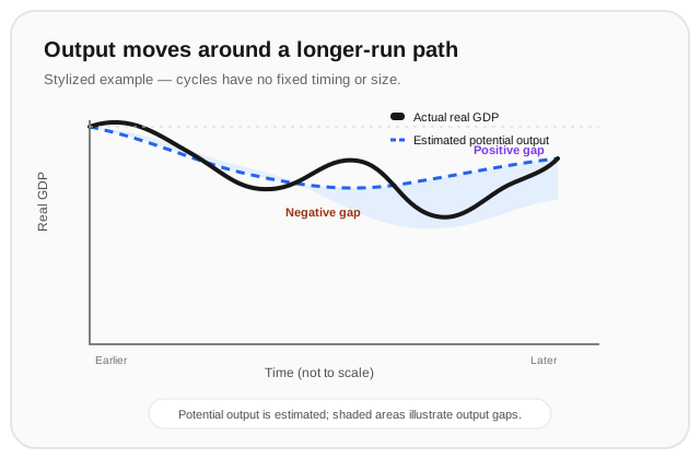
Real GDP often rises over long periods as population, skills, technology, and productive capacity change. Around that longer-run path, output can speed up or slow down. A broad period of rising economic activity is called an expansion; a broad period of weakening activity is a contraction. A recession is a substantial, widespread decline in activity, but statistical agencies and countries do not all use one identical rule to date recessions. Two consecutive quarters of falling real GDP is a familiar rule of thumb, not a universal definition.

The economy’s longer-run productive path is often called potential output. It is an estimate of what the economy could produce sustainably with its available labor, capital, and technology—not a physical speed limit that can be read from a meter. Actual output can be above or below that estimate for a time.

The output gap expresses the difference as a share of potential output:

where $Y$ is actual real GDP and $Y^*$ is estimated potential output. A negative gap means measured output is below the estimated sustainable path; a positive gap means it is above. Neither sign says every industry is in the same condition, and estimates of potential output can be revised as new data arrive.

Aggregate demand: planned spending across the economy

In a simple open-economy framework, planned expenditure on domestic output can be organized as

where $C$ is planned household consumption, $I$ is planned business investment and inventory accumulation, $G$ is government purchases of goods and services, $X$ is planned exports, and $M$ is planned imports. The expression resembles the GDP expenditure identity because, after spending and production are recorded, national accounts must reconcile the value of domestic output with the spending on it.

But there is an important distinction. The national-accounts identity records actual spending and output after the fact. In a model of aggregate demand, we may be asking about planned spending before firms know whether every good they produce will be sold. If firms produce more than buyers planned to purchase, inventories rise unexpectedly. Firms may then cut production or postpone hiring. The accounting identity still holds because inventory changes are counted as investment; the unexpected inventory accumulation is precisely the clue that plans and production did not line up as intended.

The letters are familiar from GDP, but here they help us ask how decisions change:

• Households may alter $C$ when confidence, disposable income, wealth, or borrowing conditions change.
• Firms may alter $I$ when expected sales, financing costs, or uncertainty change.
• Governments choose $G$ through purchases of goods and services; transfers affect recipients’ income but are not themselves purchases of current output.
• Foreign demand, exchange rates, and incomes abroad can change $X$ and $M$.

These categories are connected. A household’s spending is another firm’s revenue; a firm’s investment is income for the people building its equipment. A spending decline can therefore reduce someone else’s income, which may lead to another spending decline. The chain is a possibility to analyze, not a guarantee that one initial change will produce a fixed-sized outcome.

Moving along aggregate demand, or shifting it?

An aggregate-demand curve relates the overall price level to the quantity of domestic real output buyers plan to purchase, holding other influences fixed. In the standard introductory model, a lower overall price level is associated with a larger quantity of output demanded. This is not the same thing as the downward-sloping demand curve for one product: economy-wide mechanisms such as purchasing power, interest rates, and trade contribute to the relationship.

If the overall price level changes and the other influences are held fixed, the model describes a movement along the aggregate-demand curve. If household confidence changes, firms revise investment plans, government purchases change, or foreign demand changes, planned spending can change at each price level. The entire curve then shifts.

A negative spending shock—for example, households delaying purchases because they fear job loss—can shift aggregate demand left. In the short run, firms may respond to weaker sales by reducing production and hiring. Lower incomes may then weaken spending further. How much of that chain occurs depends on the causes, the timing of price and wage adjustments, the actions of firms and households, and policy responses.

Aggregate demand is not the whole economy. It organizes the spending side, but production capacity, input costs, technology, supply disruptions, expectations, and institutions also shape what happens. A sharp rise in production costs can weaken output even if spending has not fallen; a gain in productive capacity can raise potential output without a sudden spending boom. To explain a real episode, we need evidence about both demand and supply, not just a curve with a convenient label.

Why a downturn reaches more than one indicator

Suppose households and firms cut planned spending. If firms sell less than expected, they may first build inventories unintentionally. If they judge the weakness temporary, they might wait. If they expect it to last, they may scale back production, hours, and hiring. Lower employment or hours can reduce household income; weaker income can then restrain consumption.

That chain helps explain why real GDP and employment often weaken together in a contraction. It also helps explain why prices need not move in one guaranteed direction. Weaker demand may ease pressure on some prices, but supply disruptions or rising costs can push prices upward at the same time. GDP, unemployment, and inflation are connected indicators, not interchangeable readings of one hidden dial.

The relationship is not exact or immediate. Employment data can lag output; inflation can respond with delays; a recession can affect industries unevenly. And an economy’s measured output may keep rising while growing more slowly than potential—so “growth slowed” is not always the same as “output fell.” These distinctions matter whenever a headline says the economy is booming or shrinking.

Worked example

Where this leads

Business cycles connect the measures we have built so far: production can move below or above potential, employment can respond as firms adjust, and prices may react differently depending on whether demand, supply, or both are changing. The next step is to study aggregate supply and the short-run trade-offs and limits that appear when the economy’s spending changes meet its productive capacity.