Continuous-Time Optimization: Hamiltonians and Transversality

Would you rather consume an extra unit today, or leave it invested so that it can support consumption later? In a two-period model, we compared two dates. But a growing economy does not make its most important decisions only twice. Consumption and investment can change every instant, and the choice at one moment changes the resources available at all later moments. How do we optimize over a whole path without writing down infinitely many separate choices?

The answer is optimal control. It takes the intertemporal trade-off behind the Euler equation and gives us a compact language for continuous time: a state variable records what has accumulated, a control variable records what can be chosen, and a Hamiltonian combines the immediate payoff with the value of changing the state. The method is a disciplined way to derive the path—not a machine that makes assumptions disappear.

A capital-and-consumption problem

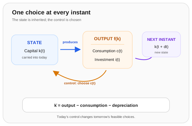
Start with a deliberately simple economy with no population or technology growth. Let $k(t)$ be capital, $c(t)$ consumption, $f(k)$ output, and $\delta$ the depreciation rate. Feasible production must be divided between consumption and investment, so capital evolves according to

\dot{k}(t)=f(k(t))-c(t)-\delta k(t).

The household values consumption over an infinite horizon:

\max_{\{c(t)\}_{t\geq 0}}\int_0^\infty e^{-\rho t}u(c(t))\,dt, \qquad \rho>0,

subject to the capital equation and given initial capital $k(0)=k_0$ . The function $u$ is increasing and concave: more consumption is better, but each extra unit adds less utility than the previous one. The discount rate $\rho$ expresses how future utility is weighted relative to current utility.

There are two kinds of variables here. Capital $k$ is the state: today’s choice changes the amount carried into tomorrow. Consumption $c$ is the control: the household chooses it at each instant. Consuming more now raises utility now but leaves less output available for capital accumulation.

A continuous-time choice diagram shows capital as a state carried forward from one instant to the next. At each date, output is divided between consumption and investment; investment changes the state, which in turn changes future output and future choices. — The state is inherited and changes through time; the control is chosen along the path. A Hamiltonian puts the current payoff and the shadow value of state accumulation into one expression.

The Hamiltonian and its first-order conditions

At a given date, one more unit of capital is not valuable merely because it exists. It is valuable because it can support future production and consumption. Let $\lambda(t)$ denote that shadow value. The present-value Hamiltonian is

H^P=e^{-\rho t}u(c)+\mu\,[f(k)-c-\delta k],

where $\mu(t)$ is a present-value costate. It is convenient to rescale the shadow value as $\lambda(t)=e^{\rho t}\mu(t)$ , giving the current-value Hamiltonian

H=u(c)+\lambda\,[f(k)-c-\delta k].

For an interior optimum, the control condition is

\frac{\partial H}{\partial c}=u'(c)-\lambda=0, \qquad\text{so}\qquad \lambda=u'(c).

This has a direct economic interpretation. If the household consumes one less unit now, it can retain one more unit of capital. The utility cost of that decision is $u'(c)$ ; the current shadow value of the extra capital is $\lambda$ . At the optimum, the two are equal. If they were not, the household could improve its plan by shifting consumption slightly.

The state equation remains the resource constraint, while the current-value costate equation is

\dot{k}=f(k)-c-\delta k, \qquad \dot{\lambda}=\rho\lambda-\frac{\partial H}{\partial k} =\bigl(\rho+\delta-f'(k)\bigr)\lambda.

Why does the costate equation contain $\rho$ ? A current-value shadow price is measured in date- $t$ utility units. It changes both because capital’s physical return changes its future usefulness and because future utility is discounted. If instead we used the present-value costate $\mu=e^{-\rho t}\lambda$ , the explicit discount term would disappear from its costate equation.

Together, the two equations describe a path: the state changes with the resources left after consumption, while the shadow value changes with the return to capital and the discount rate. These are not two independent choices. A feasible optimal path must satisfy them at every date and meet the initial condition for capital.

Recovering the Euler equation

The Hamiltonian has not replaced the intertemporal choice logic; it lets us see it operating continuously. Combine $\lambda=u'(c)$ with the costate equation. Differentiating the control condition gives

\dot{\lambda}=u''(c)\dot{c}.

Substitute $\lambda=u'(c)$ into the costate equation and divide by $u'(c)$ :

\frac{u''(c)}{u'(c)}\dot{c}=\rho+\delta-f'(k).

Define the elasticity of marginal utility, or coefficient of relative risk aversion, as

\sigma(c)=-\frac{c u''(c)}{u'(c)}>0.

Then the optimal consumption-growth condition is

\frac{\dot{c}}{c}=\frac{f'(k)-\delta-\rho}{\sigma(c)}.

For constant-relative-risk-aversion utility, $u(c)=\frac{c^{1-\sigma}-1}{1-\sigma}$ (with $u(c)=\ln c$ when $\sigma=1$ ), the coefficient is constant. If the net marginal return to capital, $f'(k)-\delta$ , exceeds the discount rate $\rho$ , the household is willing to postpone some consumption and consumption grows along the optimum. If it is lower, the path tilts toward consumption earlier. The exact path still depends on the capital equation and the boundary conditions.

This is the continuous-time cousin of the discrete Euler equation. In discrete time, we balanced marginal utility today against the discounted return to consumption tomorrow. Here, the costate tracks the value of one extra unit of capital from instant to instant, and its motion produces the same marginal trade-off.

Why local conditions are not enough

The state equation and the two first-order conditions are necessary ingredients, not a complete solution by themselves. The state has an initial value, but an infinite-horizon problem has no ordinary final date at which to specify capital. A path can satisfy every local equation and still be unacceptable if it accumulates assets that are never used, or if it relies on an ever-growing liability that can never be repaid.

A common transversality condition for this problem is

\lim_{t\to\infty}e^{-\rho t}\lambda(t)k(t)=0.

Since $\mu(t)=e^{-\rho t}\lambda(t)$ is the present-value shadow price, the condition says that the discounted value of the remaining capital stock vanishes at the horizon. It rules out leaving valuable resources permanently unused in the limit. The corresponding no-Ponzi condition rules out financing consumption with debt that is never backed by future resources.

The exact terminal condition depends on the model’s feasible set, whether the state is bounded below, and whether a finite terminal date or bequest value is present. It should not be pasted into every model without checking those assumptions. Its role is more general: local optimality must be paired with a condition that makes the whole infinite path economically meaningful.

Worked example

A household has logarithmic utility $u(c)=\ln c$ and faces the production function $f(k)=2\sqrt{k}$ . Depreciation is $\delta=0.05$ per year and the discount rate is $\rho=0.03$ . At a point on an interior optimal path where $k=100$ , find the instantaneous optimal growth rate of consumption. What does the result say—and not say—about the full path?

Step 1 — find the marginal product of capital.

f'(k)=\frac{1}{\sqrt{k}}, \qquad f'(100)=0.10.

Step 2 — use the continuous-time Euler equation. For logarithmic utility, $\sigma=1$ , so

\frac{\dot{c}}{c}=f'(k)-\delta-\rho =0.10-0.05-0.03=0.02.

At this point, optimal consumption is growing at 2% per year. The marginal product is 10%; after depreciation, capital returns 5%; the household’s 3% discount rate leaves a 2% incentive to shift consumption toward the future.

Step 3 — do not mistake a local rate for a complete solution. The 2% rate applies at the stated point, where $k=100$ . As capital changes, $f'(k)$ changes, so the growth rate generally changes too. To find the entire path, we would also need initial capital, the state equation, and the terminal/transversality condition.

Where this leads

The Hamiltonian converts a continuous stream of choices into a state equation, a costate equation, and a transversality condition. That is the mathematical bridge between the household Euler equation and a full dynamic macroeconomic model. The next step is to put optimizing households and competitive firms together: the Ramsey–Cass–Koopmans model lets consumption and capital be chosen jointly over time rather than treating the saving rate as fixed from outside.