The Ramsey–Cass–Koopmans Model: Consumption, Capital, and the Long Run

In the Solow model, the saving rate was an input: choose $s$ , and the model tells us how capital responds. But why should an economy save exactly 20% or 30%? A household that saves less consumes more now; one that saves more can consume more later. The saving rate is not an independent dial if people are choosing over time. Can we put those choices inside the growth model and still make the transition to equilibrium precise?

The Ramsey–Cass–Koopmans (RCK) model does exactly that. Households choose consumption to maximize lifetime utility, firms rent capital and labor until their marginal products equal their prices, and aggregate saving becomes investment that changes the capital stock. The economy’s saving behavior is now an outcome of preferences, technology, and initial conditions—not a parameter imposed from outside.

We begin with the deterministic, continuous-time benchmark. It is intentionally spare: one representative household, one good, competitive production, no uncertainty, and no policy distortions. These assumptions let us isolate the model’s central dynamic mechanism. We will add labor and technology growth after deriving the core system.

Resources, preferences, and competitive returns

Let $k(t)$ be capital per person and $c(t)$ consumption per person. Labor and technology are initially constant. Output per person is produced by $y=f(k)$ , where $f'>0$ and $f''<0$ : capital raises output, but diminishing returns make its marginal product fall as capital accumulates. Capital depreciates at rate $\delta$ :

\dot{k}=f(k)-c-\delta k.

The representative household chooses a consumption path to maximize

\max_{\{c(t)\}}\int_0^\infty e^{-\rho t}u(c(t))\,dt, \qquad \rho>0,

subject to the resource equation and initial capital $k(0)=k_0$ . Utility is increasing and strictly concave. The discount rate $\rho$ measures impatience; a larger $\rho$ puts more weight on consumption sooner.

Under perfect competition, a firm takes prices as given. If the production function has constant returns to scale in capital and labor, the real wage equals the marginal product of labor and the rental rate on capital equals its marginal product. In per-person notation, the gross return to capital is $f'(k)$ , so the household’s net return after depreciation is

r^k=f'(k)-\delta.

This is the connection between the production side and the household’s intertemporal choice: the return that rewards postponing consumption is generated by the economy’s current capital stock.

The Ramsey phase diagram plots capital per person horizontally and consumption per person vertically. The k-dot zero curve slopes upward; the c-dot zero curve is vertical at the steady-state capital level. Their intersection is the steady state, and a stable saddle path selects the consumption trajectory consistent with convergence. — The state variable $k$ is inherited, while consumption $c$ can jump when the economy’s outlook changes. The saddle path selects the initial consumption consistent with convergence; nearby paths generally move away from the steady state.

Derive the household’s optimal path

The current-value Hamiltonian is

H=u(c)+\lambda\,[f(k)-c-\delta k].

The control condition $u'(c)=\lambda$ equates the marginal utility of consumption to the shadow value of capital. The costate equation is

\dot{\lambda}=\bigl(\rho+\delta-f'(k)\bigr)\lambda.

Differentiate $u'(c)=\lambda$ and substitute the costate equation. If utility has constant relative risk aversion,

u(c)=\frac{c^{1-\sigma}-1}{1-\sigma}, \qquad \sigma>0,

with $u(c)=\ln c$ at $\sigma=1$ , then $u'(c)=c^{-\sigma}$ . Taking growth rates gives $\dot{\lambda}/\lambda=-\sigma\dot{c}/c$ . Therefore

\frac{\dot{c}}{c} =\frac{f'(k)-\delta-\rho}{\sigma}.

The entire equilibrium path is characterized by two coupled differential equations:

\boxed{\begin{aligned} \dot{k} &= f(k)-c-\delta k,\\ \frac{\dot{c}}{c} &= \frac{f'(k)-\delta-\rho}{\sigma}. \end{aligned}}

The first equation is resource feasibility. The second is optimality. When capital is scarce, $f'(k)$ is high, making the return to investment attractive and tilting the optimal consumption path upward. As capital accumulates, diminishing returns lower $f'(k)$ ; consumption growth slows. If the return falls below impatience, the household prefers to consume relatively more now, and consumption declines along the optimal path.

The parameter $\sigma$ is the inverse intertemporal elasticity of substitution. A larger $\sigma$ makes consumption growth less responsive to a given gap between the net return and $\rho$ . It captures curvature in preferences, not a technological limit on how fast the economy can grow.

The steady state—and why the path is a saddle

At a steady state, both variables are constant. From $\dot{c}=0$ ,

f'(k^*)=\delta+\rho.

The marginal product of capital has fallen to the point where the net return equals the household’s discount rate. From $\dot{k}=0$ ,

c^*=f(k^*)-\delta k^*.

These two conditions determine the steady-state capital stock and consumption, given the model’s parameters. Notice that the saving rate was not specified. It is whatever fraction of output is required along the equilibrium path to satisfy household optimality and the resource constraint.

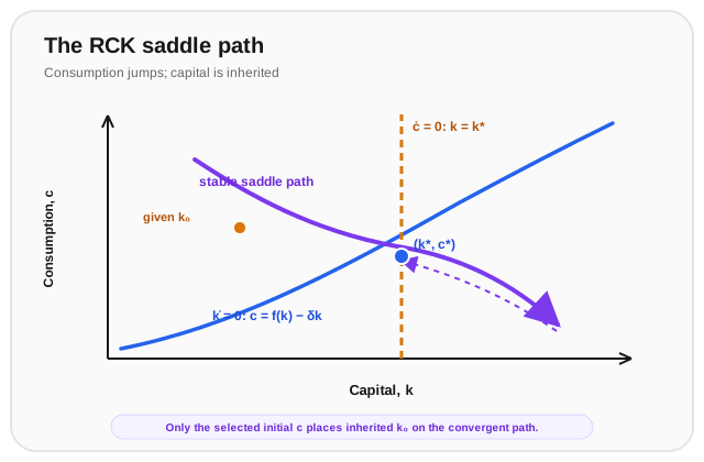
The steady state does not attract every feasible path. Capital $k$ is a state variable: its initial value is inherited and cannot jump when the model begins. Consumption $c$ is a control variable: households can adjust it immediately. If initial consumption is too high, too little is invested and capital may move away from its steady state. If it is too low, excess saving may send capital along a path that is inconsistent with optimality or the terminal condition. Only one initial consumption level—locally, on the stable arm—typically places a given initial $k_0$ on a path converging to $(k^*,c^*)$ .

This is the saddle-path property. One eigenvalue of the linearized system around the steady state is stable and another unstable; the stable manifold selects the convergent transition. The transversality condition rules out paths that satisfy the local equations but leave capital’s value unused or finance consumption with unsustainable debt. Thus the model combines an initial condition for the state with a terminal condition for the shadow value to select a unique equilibrium path under standard regularity assumptions.

A comparison with Solow and the Golden Rule

In Solow, a constant saving rate determines capital accumulation. In RCK, consumption is chosen optimally and the implied saving rate generally changes as the economy moves toward its steady state. Both frameworks use diminishing returns and a resource constraint, but they answer different questions: Solow asks what follows from a saving rule; RCK asks what path results when households choose consumption over time.

The RCK steady state need not maximize steady-state consumption. The Golden Rule capital stock solves

f'(k_{GR})=\delta,

because it maximizes $f(k)-\delta k$ in this no-growth benchmark. The RCK steady state instead satisfies $f'(k^*)=\delta+\rho$ . For positive impatience, this usually implies $k^*<k_{GR}$ under a concave production function. The household values consumption now as well as later; it does not choose capital solely to maximize the consumption level of a stationary generation.

The model’s welfare result is conditional on the assumptions that produced it. A decentralized competitive equilibrium can coincide with an efficient allocation when markets are complete and there are no externalities, market power, taxes, or other distortions. With uncertainty, incomplete insurance, borrowing constraints, heterogeneous households, or policy wedges, that conclusion needs to be re-examined rather than assumed.

Population and technology growth

The core system can be extended to a growing economy. Let labor grow at rate $n$ , technology at rate $g$ , and production be $Y=F(K,AL)$ . Define capital and consumption per effective worker as $k=K/(AL)$ and $c=C/(AL)$ . Feasibility becomes

\dot{k}=f(k)-c-(\delta+n+g)k.

The extra terms represent capital needed to replace depreciation and equip expanding effective labor. With standard CRRA preferences and the corresponding balanced-growth normalization, the consumption-growth condition in effective-worker units includes the growth adjustment:

\frac{\dot{c}}{c} =\frac{f'(k)-\delta-\rho-\sigma g}{\sigma}.

At a balanced-growth steady state in effective-worker units, $f'(k^*)=\delta+\rho+\sigma g$ . The economy can then have rising output and consumption per person because technology grows, even though $k$ and $c$ per effective worker are constant. The precise population-discount convention matters when deriving welfare weights; these equations use the common representative-household normalization in which $\rho$ is the pure rate of time preference and aggregate utility accounts for population growth.

Worked example

Consider the no-growth RCK model with $f(k)=2\sqrt{k}$ , logarithmic utility, depreciation $\delta=0.05$ , and discount rate $\rho=0.03$ . Find the steady-state capital and consumption per person. If the economy begins with $k_0=25$ , is its initial marginal product above or below the steady-state value, and what does the Euler equation imply for consumption growth on the optimal path?

Step 1 — use the steady-state return condition. Since $f'(k)=1/\sqrt{k}$ and $\sigma=1$ ,

f'(k^*)=\delta+\rho=0.08, \qquad \frac{1}{\sqrt{k^*}}=0.08.

Thus $\sqrt{k^*}=12.5$ and

k^*=156.25.

Step 2 — calculate steady-state consumption.

c^*=f(k^*)-\delta k^* =2\sqrt{156.25}-0.05(156.25) =25-7.8125=17.1875.

Step 3 — inspect the initial return. At $k_0=25$ ,

f'(25)=\frac{1}{5}=0.20,

which exceeds the steady-state marginal product of $0.08$ . For logarithmic utility, the Euler equation gives $\dot{c}/c=f'(k)-\delta-\rho$ , so at that capital stock

\frac{\dot{c}}{c}=0.20-0.05-0.03=0.12.

The optimal consumption-growth rate is 12% per year at that point. This is a local implication, not a complete transition path: to determine the initial consumption level, we must select the point on the stable saddle path that is consistent with the initial capital stock and the transversality condition.

Where this leads

The Ramsey–Cass–Koopmans model closes the loop between the household Euler equation, firms’ marginal returns, and aggregate capital accumulation. It gives us a disciplined account of a transition path and clarifies why a saving rate is an outcome rather than an input. The next research layers can relax its representative-household and certainty assumptions—introducing heterogeneous agents, incomplete markets, uncertainty, fiscal policy, and open-economy capital flows—while keeping the same dynamic-optimization core visible.