Intertemporal Choice: Consumption, Saving, and the Euler Equation

Suppose your income is high this year and expected to be lower next year. Do you spend everything now, or set some aside? Now imagine the real interest rate changes. Saving becomes more rewarding, but it also changes how wealthy you feel over your lifetime. The answer is not simply “higher interest means more saving.” We need a model of choices across time.

Intertemporal choice is the allocation of resources among different dates. A two-period model is small enough to solve on paper, yet it contains the central logic behind household saving and the Euler equation used in much more advanced macroeconomics. We will begin with certain income and a known real interest rate; uncertainty, borrowing limits, and many households will come later.

The budget across two periods

Let $y_1$ and $y_2$ be income in periods one and two, and let $c_1$ and $c_2$ be consumption. With no initial assets, a household can save or borrow in the first period. Call that amount $s$ ; a negative value means borrowing:

c_1 + s = y_1,

c_2 = y_2 + (1+r)s,

where $r$ is the real interest rate over the period. Save one unit now and it becomes $1+r$ units of consumption resources next period. Borrow one unit and the household must repay $1+r$ later.

Substitute $s=y_1-c_1$ into the second-period budget, then divide by $1+r$ and rearrange:

c_1 + \frac{c_2}{1+r} = y_1 + \frac{y_2}{1+r}.

This is the present-value budget constraint. The left side is the present value of consumption; the right side is the present value of income. The equation describes all affordable consumption plans under the assumptions that the household can borrow or save freely at the same rate and has no assets left over after period two.

A two-period timeline shows first-period income of 150, consumption of about 125.6, and saving of about 24.4. The savings earn a 5 percent real return, becoming about 25.6 in period two; together with second-period income of 100, they support consumption of about 125.6. — Saving moves purchasing power from the first period to the second. The example assumes certainty, a 5% real return, and unrestricted borrowing and saving; actual households face risk and different credit terms.

The slope of the budget line in $(c_1,c_2)$ space is $-(1+r)$ . One more unit consumed now costs $1+r$ units of future consumption, because saving that unit would have produced that return. The interest rate is therefore a relative price across time.

Preferences decide how to use the budget

Having a budget does not tell us which affordable plan the household prefers. Suppose its preferences can be represented by

U(c_1,c_2)=u(c_1)+\beta u(c_2), \qquad 0<\beta<1.

The function $u$ describes the utility from consumption in one period. The discount factor $\beta$ captures how the household weights future utility relative to present utility; a lower $\beta$ means the future is weighted less heavily in this model. It is not the same thing as the market interest rate.

The household chooses consumption to maximize $U$ subject to the present-value budget. Write the Lagrangian:

\mathcal{L}=u(c_1)+\beta u(c_2)+\lambda\left(y_1+\frac{y_2}{1+r}-c_1-\frac{c_2}{1+r}\right).

For an interior optimum, the first-order conditions are

u'(c_1)=\lambda, \qquad \beta u'(c_2)=\frac{\lambda}{1+r}.

Eliminate $\lambda$ and we get the Euler equation:

u'(c_1)=\beta(1+r)u'(c_2).

This equation is a balance at the margin. If the household reduces consumption by one unit now, it gives up $u'(c_1)$ units of current utility, but can gain $1+r$ units of future consumption, worth $\beta(1+r)u'(c_2)$ in discounted utility. At the optimum, those two effects balance. The Euler equation is not a law that consumption must be equal; it is a condition describing an optimizing choice under the stated assumptions.

Patience and the shape of consumption over time

For constant-relative-risk-aversion preferences, a common form is

u(c)=\frac{c^{1-\sigma}-1}{1-\sigma}, \qquad \sigma>0,

with logarithmic utility $u(c)=\ln c$ when $\sigma=1$ . Its marginal utility is $u'(c)=c^{-\sigma}$ . Substitute that into the Euler equation:

c_1^{-\sigma}=\beta(1+r)c_2^{-\sigma},

so the optimal consumption ratio is

\frac{c_2}{c_1}=\left[\beta(1+r)\right]^{1/\sigma}.

If $\beta(1+r)=1$ , the household chooses equal consumption across the two periods in this simple model. If it is greater than one, the model favors more consumption later; if it is less than one, more consumption now. The parameter $\sigma$ controls how sharply the household wants to smooth consumption: a larger value makes the ratio respond less to a given change in $\beta(1+r)$ .

This is why “patience” and “interest rates” cannot be discussed separately. A patient household may save even at a modest return; a high return can make delayed consumption attractive even for a less patient household. But lifetime income and where it arrives also matter for the actual amount saved.

Why a higher real rate has no guaranteed saving effect

A rise in $r$ changes the relative price between today and tomorrow. That creates a substitution effect: future consumption now costs less in terms of current consumption, so a household may shift toward saving. This is the channel often emphasized in simple explanations.

There is also an income effect. A household that already saves gains more future resources from its existing assets and may choose to consume more in both periods. A borrower, by contrast, faces a higher repayment cost and may feel poorer. These effects can point in different directions. Therefore, the change in one household’s saving is not determined by the interest rate alone, and the effect on total national saving is even less automatic.

The model also assumes that people can borrow and save at the same rate. In reality, a household may face a high loan rate, a low deposit rate, fees, collateral requirements, or no access to credit at all. A borrowing constraint can prevent someone from choosing the smooth consumption path that would maximize their modeled utility. Income risk, unemployment, health, family obligations, taxes, and precautionary motives also matter.

Finally, individual saving is not identical to investment in GDP. A household’s deposit or bond purchase is a financial decision; national-accounts investment counts newly produced capital goods, housing, and inventory changes. Financial markets can connect the two, while the national saving–investment identities describe the economy-wide totals after the accounts are recorded.

Worked example

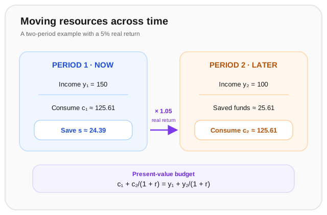
A household expects income of 150 units now and 100 units next period. The real interest rate is 5%, and its discount factor is $\beta=1/1.05$ . It has logarithmic utility, $U=\ln c_1+\beta\ln c_2$ , and can borrow or save freely. Find the optimal consumption ratio, the present value of lifetime resources, and the household’s saving in period one.

Step 1 — use the Euler equation for log utility. Since $u'(c)=1/c$ , the Euler equation gives

\frac{1}{c_1}=\beta(1+r)\frac{1}{c_2}.

Here $\beta(1+r)=(1/1.05)(1.05)=1$ , so $c_2/c_1=1$ . The household chooses equal consumption across the two dates.

Step 2 — calculate lifetime resources in present-value terms.

W=150+\frac{100}{1.05}\approx245.24.

The present value of consumption must equal $W$ . Since $c_1=c_2=c$ ,

c+\frac{c}{1.05}=245.24, \qquad c\approx125.61.

Step 3 — find first-period saving. The first-period budget is $c_1+s=y_1$ , so

s=150-125.61\approx24.39.

The household saves about 24.39 units now. At 5%, that becomes about $24.39(1.05)\approx25.61$ next period; adding future income of 100 gives consumption of about 125.61. The household shifts resources across time to smooth consumption, given its preferences and the assumptions of the example.

Where this leads

The Euler equation turns the saving decision into a precise trade-off between marginal utility today and tomorrow. In the next layer, the Ramsey–Cass–Koopmans model puts this household choice inside a growing economy: consumption is chosen over time, firms produce output, and saving determines capital accumulation rather than being fixed from outside. That is the bridge from introductory growth models to dynamic macroeconomics.