Free Energy and Thermodynamic Potentials

The second law says entropy increases for an isolated system. That's a clean, powerful statement — and almost useless for the actual experiments physicists and chemists run every day. A beaker of reacting chemicals on a lab bench is not isolated. It sits in a room at a fixed temperature, freely trading heat with the air around it, and it's often open to the atmosphere, freely trading volume against a fixed external pressure too. The system you actually care about is only ever part of "the isolated universe" the second law talks about — so what quantity should you actually track, if not the entropy of a system that isn't isolated to begin with?

There is an answer, and it isn't a retreat from the second law — it's the second law, worked out honestly for a system that isn't alone.

Building the right quantity from the second law itself

Consider a system held at fixed temperature $T$ by contact with a large reservoir (a room, a water bath — anything big enough that its own temperature doesn't budge), and fixed volume $V$ (a rigid, sealed container: no work is done by expansion). The full second law applies to the combined system-plus-reservoir, since that combination really is isolated:

\Delta S_{\text{sys}} + \Delta S_{\text{res}} \geq 0

At fixed volume, the system does no work, so whatever energy it gains comes entirely as heat: $\Delta U_{\text{sys}} = Q_{\text{sys}}$ . Whatever heat flows into the system leaves the reservoir, so $Q_{\text{res}} = -Q_{\text{sys}} = -\Delta U_{\text{sys}}$ , and because the reservoir is so large that this heat exchange happens at its fixed temperature $T$ , its entropy change is exactly $\Delta S_{\text{res}} = Q_{\text{res}}/T = -\Delta U_{\text{sys}}/T$ . Substitute into the second law:

\Delta S_{\text{sys}} - \frac{\Delta U_{\text{sys}}}{T} \geq 0

Multiply through by $-T$ (which is positive, so the inequality flips direction):

\Delta U_{\text{sys}} - T\Delta S_{\text{sys}} \leq 0

The left side is exactly $\Delta(U-TS)$ , evaluated for the system alone. Define the Helmholtz free energy:

F \equiv U - TS

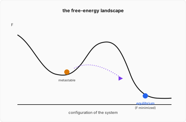
and the result reads $\Delta F \leq 0$ . At fixed temperature and volume, a system evolves so as to decrease its free energy, and sits in equilibrium exactly where $F$ is minimized. The second law, which looked like a statement about the entire universe's entropy, has become a statement purely about the system itself — provided you track $F$ , not $S$ , once the system is embedded in a reservoir rather than isolated.

The identical argument, run at fixed temperature and fixed pressure instead of fixed volume (an open beaker exposed to the atmosphere, rather than a sealed rigid box, so the system can also do $P\Delta V$ work against the surrounding air as it changes volume) produces a close cousin, the Gibbs free energy:

G \equiv U + PV - TS = H - TS

where $H\equiv U+PV$ is the enthalpy. Exactly as with $F$ , a system held at fixed $T$ and $P$ evolves to minimize $G$ . The two potentials aren't competing ideas — they're the same construction, applied to two different sets of experimental constraints. Constant volume, sealed container: use $F$ . Constant pressure, open to the atmosphere: use $G$ . Almost every real chemical reaction happening in an open flask is a $G$ -minimization problem; almost every gas confined to a rigid tank is an $F$ -minimization problem.

A curve representing free energy F plotted against some configuration variable of the system, shaped like a valley with two local dips of different depths, with a small ball resting partway up the shallower dip and an arrow showing it rolling downhill toward the deeper, global minimum, labeled equilibrium.

A system in contact with a reservoir rolls downhill on the free-energy landscape exactly the way a ball rolls downhill on an ordinary potential-energy landscape — except here, "downhill" already has entropy baked into its definition.

The bridge to the partition function

This is the moment the partition function earns the central role it was given. Recall the Gibbs entropy formula, the natural generalization of Boltzmann's $S=k_B\ln\Omega$ to a system whose microstates aren't all equally likely, only distributed according to some probability $P_s$ :

S = -k_B\sum_s P_s\ln P_s

As a sanity check before using it: if every one of $\Omega$ microstates is equally likely, $P_s = 1/\Omega$ for each, this reduces to $S = -k_B\sum_s\frac{1}{\Omega}\ln\frac{1}{\Omega} = -k_B\cdot\Omega\cdot\frac{1}{\Omega}\cdot(-\ln\Omega) = k_B\ln\Omega$ — exactly Boltzmann's formula recovered as the special case of equal probabilities.

Now use the actual Boltzmann distribution, $P_s = e^{-\beta E_s}/Z$ , so that $\ln P_s = -\beta E_s - \ln Z$ . Substitute directly:

S = -k_B\sum_s P_s\left(-\beta E_s - \ln Z\right) = k_B\beta\sum_s P_s E_s + k_B\ln Z\sum_s P_s

The first sum is exactly $\langle E\rangle$ by definition, and the second sum is $1$ since probabilities add up to one. With $k_B\beta = 1/T$ :

S = \frac{\langle E\rangle}{T} + k_B\ln Z

Rearranging, using $U=\langle E\rangle$ :

TS = U + k_BT\ln Z \quad\Longrightarrow\quad U - TS = -k_BT\ln Z

The left side is exactly $F$ . So:

\boxed{F = -k_BT\ln Z}

The Helmholtz free energy is nothing but the partition function, logarithmed and rescaled. Every thermodynamic quantity this track has built — average energy, entropy, and now free energy — is obtainable from $Z$ alone by ordinary calculus: $U=-\partial\ln Z/\partial\beta$ , $S = (U-F)/T$ , and $F$ itself directly from $Z$ with no further work.

Worked example

Using the two-level system from the previous topic, with energies $0$ and $\varepsilon$ and partition function $Z=1+e^{-\beta\varepsilon}$ , find the Helmholtz free energy $F(T)$ , then extract the entropy $S(T)$ from it. Check the $T\to0$ and $T\to\infty$ limits. (click to reveal the solution)

Free energy, directly from $F=-k_BT\ln Z$ :

F(T) = -k_BT\ln\left(1+e^{-\varepsilon/k_BT}\right)

Extracting entropy, using the general relation just derived, $S = (U-F)/T$ , together with the average energy already found in the previous topic, $U=\langle E\rangle = \varepsilon/(e^{\beta\varepsilon}+1)$ :

S = \frac{U-F}{T} = \frac{1}{T}\left[\frac{\varepsilon}{e^{\varepsilon/k_BT}+1} + k_BT\ln\left(1+e^{-\varepsilon/k_BT}\right)\right]

S = \frac{\varepsilon}{T\left(e^{\varepsilon/k_BT}+1\right)} + k_B\ln\left(1+e^{-\varepsilon/k_BT}\right)

Checking $T\to0$ : as $T\to0$ , $\varepsilon/k_BT\to\infty$ , so $e^{-\varepsilon/k_BT}\to0$ . The logarithm term $\to k_B\ln(1)=0$ . The first term: $e^{\varepsilon/k_BT}$ blows up in the denominator far faster than the explicit $T$ in front shrinks it, so the whole first term $\to0$ as well (an exponential beats any power of $T$ ). So $S\to0$ — exactly what the third law demands: the system is frozen into its unique, non-degenerate ground state, energy $0$ , with $\Omega=1$ and therefore zero entropy.

Checking $T\to\infty$ : as $T\to\infty$ , $\varepsilon/k_BT\to0$ , so $e^{-\varepsilon/k_BT}\to1$ , and the logarithm term $\to k_B\ln(2)$ . The first term has $e^{\varepsilon/k_BT}\to1$ , so it becomes $\varepsilon/(2T)\to0$ as $T\to\infty$ . So:

S \to k_B\ln 2

This is exactly the entropy of a two-state system with both states equally likely — $\Omega=2$ accessible microstates, each with probability $\frac12$ , giving $S=k_B\ln\Omega=k_B\ln 2$ straight from Boltzmann's original formula. At high temperature, the system stops caring about the energy difference $\varepsilon$ between its two states entirely and populates both equally — the maximum possible entropy a single two-state system can have, recovered here as a limit of the exact free-energy calculation rather than assumed in advance.

Where this leads

Free energy is the tool that finally makes the second law usable in the lab, not just in a textbook proof about isolated universes — and the identity $F=-k_BT\ln Z$ means every free-energy calculation is, underneath, just a partition-function calculation. One loose thread remains, and it's been sitting in plain sight since the very first topic in the quantum track of this curriculum: angular momentum and spin and quantum field theory both promised that spin determines whether a particle is a boson or a fermion, and both left the consequence of that distinction unexplored. It turns out bosons and fermions don't just differ in a quantum number — they populate energy levels according to two completely different statistical distributions, and the final topic in this track derives exactly what those distributions are, and exactly how the Boltzmann distribution built here turns out to be a special limiting case of both.