Quantum Statistics: Bose-Einstein and Fermi-Dirac Distributions

Two promises have been sitting unfulfilled since earlier in this curriculum. Angular momentum and spin closed by saying spin "determines whether a particle is a fermion or a boson," without saying what that determination actually changes. Quantum field theory went further, and proved — from nothing but the commutator algebra of creation operators — that swapping two identical bosons leaves a quantum state completely unchanged as a vector, not merely indistinguishable in principle. Both statements were dropped in passing, promissory notes against a payoff that hadn't been built yet. This topic cashes them in.

Here's the question that makes the payoff concrete. Put two identical particles into a system with two available energy states. How many physically distinct ways can you do that? If you learned to count in ordinary probability — flip two coins, roll two dice — your instinct says: label the particles $A$ and $B$ , and count every assignment of each one to a state separately. That instinct is about to be shown wrong, twice over, in two different directions, depending on what kind of particle you're holding.

Why identical particles aren't like labeled balls

Classically, nothing stops you from painting a tiny " $A$ " on one gas molecule and a " $B$ " on another, then tracking which is where. Quantum mechanically, this is not merely impractical — it's meaningless. Two electrons are not merely hard to tell apart; there is no experiment, even in principle, that could distinguish "electron $A$ in state $1$ , electron $B$ in state $2$ " from "electron $B$ in state $1$ , electron $A$ in state $2$ ." These are not two different physical situations that happen to look the same. They are the same situation, counted once, not twice.

That much is common to every kind of identical quantum particle. What splits particles into two genuinely different families is what happens when you ask whether two identical particles can occupy the same single-particle state at once.

Fermions — particles with half-integer spin, like the electron — obey the Pauli exclusion principle: no two identical fermions can ever occupy the same quantum state. Not "rarely." Never, under any circumstances. This is why electrons in an atom stack into shells instead of all collapsing into the lowest-energy orbital, and it is ultimately why matter takes up space at all — you cannot push through another block of atoms because doing so would force electrons into already-occupied states.

Bosons — particles with integer spin, like the photon — carry no such restriction. Any number of identical bosons can pile into the exact same state, with no penalty at all. This is why a laser can concentrate an enormous number of photons into a single mode with a single, sharply defined frequency and phase, something no assembly of fermions could ever do.

Counting states the right way: Fermi-Dirac

Take a large system of identical particles distributed among a set of single-particle energy levels $\varepsilon_i$ , and suppose level $i$ has $g_i$ distinct available quantum states at that energy (its degeneracy) hosting $n_i$ particles. For fermions, filling $n_i$ of the $g_i$ available states (each state holding $0$ or $1$ particle, never more) is exactly the combinatorics problem of choosing which states are occupied:

W_i^{\text{FD}} = \binom{g_i}{n_i} = \frac{g_i!}{n_i!(g_i-n_i)!}

The total number of microstates for the whole system is $\Omega = \prod_i W_i$ , and, exactly as in microstates and entropy, the equilibrium distribution is the one that maximizes $\ln\Omega$ , subject to fixed total particle number $N=\sum_i n_i$ and fixed total energy $E=\sum_i n_i\varepsilon_i$ .

Apply Stirling's approximation, $\ln n! \approx n\ln n - n$ , to each factorial in $\ln W_i^{\text{FD}}$ :

\ln W_i^{\text{FD}} \approx \big[g_i\ln g_i - g_i\big] - \big[n_i\ln n_i - n_i\big] - \big[(g_i-n_i)\ln(g_i-n_i)-(g_i-n_i)\big]

The three linear terms $-g_i+n_i+(g_i-n_i)$ cancel exactly, leaving:

\ln W_i^{\text{FD}} \approx g_i\ln g_i - n_i\ln n_i - (g_i-n_i)\ln(g_i-n_i)

Maximize $\sum_i \ln W_i^{\text{FD}}$ subject to the two constraints using Lagrange multipliers $\alpha$ (for fixed $N$ ) and $\beta$ (for fixed $E$ , the same $\beta=1/k_BT$ from the Boltzmann distribution) — that is, set $\partial/\partial n_i$ of $\ln\Omega - \alpha\sum_i n_i - \beta\sum_i n_i\varepsilon_i$ to zero for each $i$ :

\frac{\partial \ln W_i^{\text{FD}}}{\partial n_i} = -\ln n_i - 1 + \ln(g_i-n_i)+1 = \ln\frac{g_i-n_i}{n_i}

\ln\frac{g_i-n_i}{n_i} - \alpha - \beta\varepsilon_i = 0 \quad\Longrightarrow\quad \frac{g_i-n_i}{n_i} = e^{\alpha+\beta\varepsilon_i} \quad\Longrightarrow\quad \frac{g_i}{n_i} = 1+e^{\alpha+\beta\varepsilon_i}

Solve for $n_i$ , and write $\alpha \equiv -\mu/k_BT$ (this defines the chemical potential $\mu$ , the standard bookkeeping constant for a system with variable particle number):

\boxed{n_i = \frac{g_i}{e^{(\varepsilon_i-\mu)/k_BT}+1}}

This is the Fermi-Dirac distribution. The average occupation of a single state at energy $\varepsilon$ is $n(\varepsilon) = 1/(e^{(\varepsilon-\mu)/k_BT}+1)$ , and notice it can never exceed $1$ , no matter how low $\varepsilon$ is or how large $\beta$ gets — exactly the mathematical fingerprint of Pauli exclusion baked into the formula.

Counting states the right way: Bose-Einstein

For bosons, there's no restriction on how many particles share a state, so counting the ways to distribute $n_i$ indistinguishable particles among $g_i$ states is the standard "stars and bars" combinatorics problem:

W_i^{\text{BE}} = \binom{n_i+g_i-1}{n_i} = \frac{(n_i+g_i-1)!}{n_i!(g_i-1)!}

For large $n_i,g_i$ the $-1$ is negligible, and the identical Stirling-and-Lagrange-multiplier procedure (differentiating $\ln W_i^{\text{BE}} \approx (n_i+g_i)\ln(n_i+g_i)-n_i\ln n_i - g_i\ln g_i$ with respect to $n_i$ ) gives:

\frac{\partial\ln W_i^{\text{BE}}}{\partial n_i} = \ln(n_i+g_i) - \ln n_i = \ln\frac{n_i+g_i}{n_i}

\ln\frac{n_i+g_i}{n_i} = \alpha+\beta\varepsilon_i \quad\Longrightarrow\quad \frac{g_i}{n_i} = e^{\alpha+\beta\varepsilon_i}-1

\boxed{n_i = \frac{g_i}{e^{(\varepsilon_i-\mu)/k_BT}-1}}

This is the Bose-Einstein distribution — identical to the Fermi-Dirac result except for a single flipped sign, that $-1$ in the denominator in place of $+1$ . That tiny sign is the entire mathematical content of "bosons are allowed to pile up": as $\varepsilon_i\to\mu$ , the Fermi-Dirac denominator approaches $2$ (a finite, bounded occupation), while the Bose-Einstein denominator approaches $0$ — the occupation number can grow without bound, exactly the pileup that makes a laser, or a Bose-Einstein condensate, possible in the first place.

Three panels, one per statistics type. Left, labeled classical: two energy levels, one lower and one upper, with two distinguishable dots labeled A and B, and a tally showing four distinct arrangements. Middle, labeled bosons: two energy levels with two identical amber dots shown piled together in the lower level as one representative configuration, and a tally showing three distinct configurations. Right, labeled fermions: two energy levels with exactly one purple dot in the lower level and one in the upper level, the only allowed arrangement, and a tally showing exactly one configuration, with a note reading Pauli exclusion forces this. — Same two particles, same two energy levels, three different answers for how many distinct arrangements are physically possible — the entire content of quantum statistics is hiding in that difference.

Boltzmann as the common limit

Now take both formulas to the regime where the occupation of every state is small, $n_i/g_i \ll 1$ — physically, a low density of particles spread across many available states, or a high enough temperature that particles rarely compete for the same state. In that limit $e^{(\varepsilon_i-\mu)/k_BT} \gg 1$ , so the $\pm1$ in each denominator becomes negligible compared to the exponential itself:

n_i \approx g_i\,e^{-(\varepsilon_i-\mu)/k_BT}

for both distributions simultaneously — the $+1$ that enforced exclusion and the $-1$ that allowed pileup both wash out once occupation numbers are small enough that the particles are rarely, if ever, competing for the same state to begin with. This is exactly the classical Boltzmann distribution from earlier in this track, $n_i \propto g_i e^{-\varepsilon_i/k_BT}$ , recovered here as the common high-temperature, low-density limit of the two quantum statistics. The distinction between fermions and bosons — so absolute at low temperature and high density that it decides whether matter can hold itself up or collapse into a single state — becomes physically invisible once particles are dilute and hot enough to rarely find themselves competing for the same state. This is precisely why ordinary air, at room temperature and atmospheric pressure, is accurately described by the plain Maxwell-Boltzmann statistics from earlier in this track: its molecules are simply too dilute, and its temperature too high, for the underlying quantum statistics to show through.

Worked example

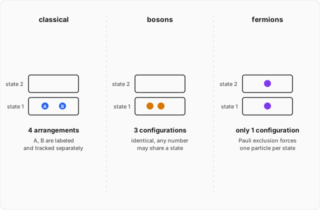
Two identical particles are to be placed among two available energy states. Enumerate the allowed configurations if the particles are (a) classical and distinguishable, (b) identical bosons, and (c) identical fermions, and compare the counts. (click to reveal the solution)

(a) Classical, distinguishable particles. Label the two particles $A$ and $B$ , and the two states $1$ and $2$ . Each particle independently can be in either state, giving $2\times2=4$ distinct arrangements:

(A{:}1,\,B{:}1), \quad (A{:}1,\,B{:}2), \quad (A{:}2,\,B{:}1), \quad (A{:}2,\,B{:}2)

All four are counted as physically different situations, because $A$ and $B$ are (by assumption) genuinely distinguishable labels.

(b) Identical bosons. Now $A$ and $B$ can no longer be told apart — only the occupation numbers $(n_1,n_2)$ , how many particles are in each state, matter. The allowed occupation patterns for $2$ particles across $2$ states are:

(n_1,n_2) = (2,0), \quad (1,1), \quad (0,2)

Exactly $3$ distinct configurations — one fewer than the classical count, because $(A{:}1,B{:}2)$ and $(A{:}2,B{:}1)$ , genuinely different classically, have collapsed into the single indistinguishable configuration $(1,1)$ .

(c) Identical fermions. Pauli exclusion forbids more than one particle per state, so $(2,0)$ and $(0,2)$ are both forbidden outright. Only one occupation pattern survives:

(n_1,n_2) = (1,1)

Exactly $1$ configuration — the two particles are forced to occupy the two different states, with no freedom left at all.

Comparing the three counts: $4$ (classical) versus $3$ (bosons) versus $1$ (fermion) — for the exact same physical setup, two particles and two states. Since the two states are equal in energy here, the equal-a-priori-probability postulate from microstates and entropy applies directly within each statistics: every allowed configuration in a given column is equally likely. That has a striking consequence. Classically, the probability of finding both particles in the same state is $2/4 = \frac12$ (the outcomes $(2,0)$ and $(0,2)$ , out of four total). For bosons, treating all $3$ allowed configurations as equally likely, that probability rises to $2/3$ — bosons genuinely prefer to bunch together, a real, measurable effect (behind, for instance, the tendency of photons to clump into the same laser mode). For fermions, the probability of both particles sharing a state is exactly $0$ — not merely small, but completely excluded by the counting itself.

Where this leads

This closes out the full arc of this track: pressure and temperature emerged from mechanics in the first topic, the exact shape of molecular speeds followed from isotropy and independence in the second, entropy emerged from counting in the third, the Boltzmann distribution and its partition function organized all of equilibrium statistical mechanics around a single sum in the fourth, the laws of thermodynamics turned out to be that same physics wearing formal names in the fifth, free energy made the second law usable for real, non-isolated systems in the sixth — and here, finally, the deepest fact about identical quantum particles, foreshadowed all the way back in angular momentum and spin and proven rigorously in quantum field theory, turns out to rewrite the statistics of matter itself, with ordinary classical statistics surviving only as the dilute, hot limit where quantum identity stops mattering. Everything in this track was, from the very first topic, the same question asked at greater and greater depth: given a huge number of possibilities, which ones actually happen — and how many ways can they happen at all.