Interacting Fields and Perturbation Theory

Go back and look hard at what quantum field theory actually built. It quantized one scalar field, found a Hamiltonian that was an infinite stack of independent oscillators, and showed that climbing a rung on any one of those oscillator-ladders is what "creating a particle" means. That was a real, complete calculation — every step checked, nothing hand-waved. But sit with what kind of universe it describes. The Hamiltonian was

\hat H = \sum_k \omega_k\left(\hat a_k^{\dagger}\hat a_k + \frac12\right),

and every term in that sum involves one mode's raising operator acting on that same mode's lowering operator. Nothing in $\hat H$ ever takes a quantum out of mode $k_1$ and puts it into mode $k_2$ . Nothing ever takes two separate particles and merges them into one, or splits one particle into two. The number of particles in every single mode is separately, exactly conserved for all time. Two electrons fired at each other in this theory would sail through each other's location without so much as noticing — no scattering, no repulsion, no collision at all. An unstable particle would never decay, because decay means one particle's quantum disappearing while several others appear, and that process simply is not written anywhere in $\hat H$ . The free field is a perfectly solved, perfectly boring universe: an infinite orchestra of oscillators, each playing forever, none of them ever influencing any other.

Real physics is not like that. Electrons repel. Photons scatter off electrons. Muons decay into electrons and neutrinos. Two protons slammed together at the LHC come apart into a spray of new particles that were not there a moment before. Every one of those processes requires modes of the field to talk to each other — for a quantum in one mode to be able to disappear while quanta in other modes appear. The free Lagrangian has no mechanism for that conversation to happen. Something has to be added.

Adding a term the free theory doesn't have

Classical field theory established that the Lagrangian density $\mathcal{L}$ is the one object that determines everything about a field's dynamics — plug it into the field Euler-Lagrange equation and out comes the equation of motion; plug it into canonical quantization and out comes the full quantum theory. The free scalar field's Lagrangian density, quantized in the previous topic, was

\mathcal{L}_0 = \frac12\dot\phi^2 - \frac12(\nabla\phi)^2 - \frac12 m^2\phi^2.

Every term here is quadratic in $\phi$ — and that is exactly why the theory was exactly solvable. A Lagrangian built purely from quadratic terms always produces linear equations of motion, and linear equations are precisely the ones that decompose into independent, uncoupled normal modes, one per momentum $k$ , with no mode ever feeding into another. Quadratic Lagrangian, independent oscillators, exact solution — the three facts are really one fact seen three ways.

To get modes talking to each other, the Lagrangian needs a term of higher order in $\phi$ . The simplest honest choice, and the one most textbooks reach for first, is a quartic self-interaction:

\mathcal{L} = \underbrace{\frac12\dot\phi^2 - \frac12(\nabla\phi)^2 - \frac12 m^2\phi^2}_{\mathcal{L}_0,\ \text{free}} \;-\; \underbrace{\frac{\lambda}{4!}\phi^4}_{\mathcal{L}_{\text{int}},\ \text{interaction}}.

The constant $\lambda$ is the coupling constant: it sets how strongly the field interacts with itself, and if you set $\lambda=0$ the whole apparatus of this topic switches off and you are back to the exactly-solved free field. The factor $4!=24$ is a bookkeeping convention (it cancels combinatorial factors that appear later, when four identical field operators in $\phi^4$ get paired up in every possible way) and carries no independent physics. Physically, this term describes a process where field quanta interact four at a time: two incoming particles meet at a point and two particles emerge, or one particle splits into three, or four particles annihilate into the vacuum — every process consistent with the four powers of $\phi$ sitting at one spacetime point. QED, built out of an electron field and a photon field talking to each other, uses a different, physically motivated interaction term (the subject of two topics from now) — but the $\phi^4$ term is the cleanest possible toy for learning how the machinery of an interacting theory actually works, and everything derived here carries over unchanged in spirit.

Why "exactly solvable" ends here

With $\mathcal{L}_{\text{int}}\neq 0$ , the field equation picks up a nonlinear term ( $\phi^3$ , from varying $\phi^4$ ), and the clean plane-wave mode expansion that made the free theory work — $\phi = \sum_k \frac{1}{\sqrt{2\omega_k V}}(a_k e^{i(k\cdot x-\omega_k t)} + \text{h.c.})$ , each mode evolving independently forever — is no longer a solution of anything. The Hamiltonian built from this $\mathcal{L}$ contains a term $\frac{\lambda}{4!}\int d^3x\,\hat\phi(x)^4$ , and expanding $\hat\phi(x)^4$ in creation and annihilation operators produces every possible combination of four $\hat a_k$ 's and $\hat a_k^\dagger$ 's, all summed together — exactly the mode-mixing that was physically required, and exactly what makes the algebra that produced clean, closed-form energy eigenstates in the free theory fail here. There is, in general, no way to diagonalize this Hamiltonian exactly. This is not a failure of cleverness; interacting quantum field theories with a genuine nonlinear term essentially never admit an exact solution, in three spatial dimensions, for any interaction anyone has found physically relevant.

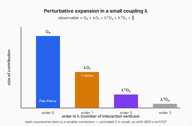
So a different strategy is needed: don't solve the interacting theory exactly. Solve it approximately, as a correction to the free theory we already solved completely, organized as a power series in the coupling constant $\lambda$ . If $\lambda$ is small, the zeroth-order answer (pure free theory, no interaction) should be close to right, the first-order correction (one factor of $\lambda$ ) should be a small refinement, the second-order correction (one factor of $\lambda^2$ ) smaller still, and so on. This is perturbation theory: treat the hard, unsolvable piece of the problem as a small nudge on top of an easy, exactly-solved piece, and compute the nudge order by order. It is one of the most heavily used tools in all of physics, and — before facing it in its full field-theoretic form — it is worth seeing stripped down to an algebra problem simple enough to solve twice, once approximately and once exactly, and to compare the two answers directly.

A bar chart with the horizontal axis labeled by increasing powers of the coupling constant, order 0, order 1, order 2, order 3, and vertical bars shrinking rapidly in height from left to right, illustrating that each successive term in a perturbative expansion contributes a smaller correction than the last, provided the coupling constant is small. — A perturbative expansion in powers of a small coupling: order zero is the exactly-solved free theory, and each higher power of the coupling adds a shrinking correction — shrinking only as long as the coupling really is small enough for the series to behave.

Worked example

Solve $x^2 + \epsilon x - 1 = 0$ perturbatively, to first order in the small parameter $\epsilon$ , and check the result against the exact quadratic formula. (click to reveal the solution)

Setting up: at $\epsilon=0$ this is trivially solvable: $x_0^2-1=0$ , giving $x_0=\pm1$ exactly — this is the "free theory" of the problem, solved completely, with no approximation anywhere. Take the branch $x_0=+1$ and ask how the small term $\epsilon x$ nudges it.

The perturbative ansatz: assume the exact root can be written as a power series in $\epsilon$ ,

x(\epsilon) = x_0 + \epsilon x_1 + \epsilon^2 x_2 + \cdots,

with $x_0=1$ already fixed, and $x_1, x_2,\ldots$ unknown coefficients to be found order by order.

Substituting into the equation and keeping only terms up to first order in $\epsilon$ (dropping $\epsilon^2$ and higher, since at this order they don't yet matter):

(x_0+\epsilon x_1)^2 + \epsilon(x_0+\epsilon x_1) - 1 = 0

\Longrightarrow\quad x_0^2 + 2\epsilon x_0 x_1 + \epsilon x_0 - 1 + O(\epsilon^2) = 0.

Collecting by power of $\epsilon$ . This equation must hold for every small $\epsilon$ , which is only possible if the coefficient of each power of $\epsilon$ vanishes separately — that is the entire logical engine of perturbation theory, in one line.

Order $\epsilon^0$ : $\quad x_0^2 - 1 = 0$ , which is exactly the free-theory equation already solved: $x_0=1$ .

Order $\epsilon^1$ : $\quad 2x_0x_1 + x_0 = 0$ .

Solving the first-order equation. This is now just linear algebra for the unknown $x_1$ , using the already-known value $x_0=1$ :

2(1)x_1 + 1 = 0 \quad\Longrightarrow\quad x_1 = -\frac12.

So, to first order in $\epsilon$ ,

\boxed{x(\epsilon) \approx 1 - \frac{\epsilon}{2}.}

Checking against the exact answer. The quadratic formula gives the exact root on this branch as

x(\epsilon) = \frac{-\epsilon+\sqrt{\epsilon^2+4}}{2} = -\frac{\epsilon}{2} + \sqrt{1+\frac{\epsilon^2}{4}}.

Expand the square root with the binomial approximation $\sqrt{1+u}\approx 1+\frac{u}{2}$ for small $u$ , here $u=\epsilon^2/4$ :

x(\epsilon) \approx -\frac{\epsilon}{2} + \left(1+\frac{\epsilon^2}{8}\right) = 1 - \frac{\epsilon}{2} + \frac{\epsilon^2}{8}.

The perturbative answer $1-\epsilon/2$ matches the exact expansion exactly through first order in $\epsilon$ — the discrepancy is $\epsilon^2/8$ , a second-order effect the first-order calculation was never claiming to capture. Carrying the perturbative expansion to order $\epsilon^2$ (repeating the same collect-and-solve procedure one power higher) would reproduce that term too.

The moral, mapped onto field theory. Three features of this toy calculation are exactly the features of the field-theoretic expansion sketched above, term by term:

Order $\epsilon^0$ is the exactly-solved free problem. Here it was $x_0^2-1=0$ ; in the field theory it is the free Lagrangian $\mathcal{L}_0$ , already fully quantized in quantum field theory.
Each order's equation uses only the previous orders' already-known solutions as input, then solves one new linear equation for the next unknown. Here, $x_1$ 's equation used the known value $x_0=1$ ; in the field theory, the $n^{\text{th}}$ -order term in $\lambda$ is built from $n$ insertions of the interaction, evaluated using the free theory's already-solved particle states.
The expansion is trustworthy only while the small parameter is actually small. If $\epsilon$ were of order $10$ rather than a small fraction, $1-\epsilon/2$ would be a poor approximation to the true root, and no finite number of extra terms would rescue a badly-behaved series. The same honest caveat applies to $\lambda$ : QED's expansion parameter, the fine-structure constant $\alpha\approx 1/137$ , is small enough that a few orders of perturbation theory give spectacular precision (the subject of two topics from now); the strong force's coupling is not nearly so forgiving at everyday energies, and perturbation theory in its bare form fails there for reasons the Standard Model topic will be honest about.

The structure of the field-theoretic expansion

The full machinery that carries out this same collect-and-solve logic for an interacting quantum field is called the Dyson series, and deriving it in full is genuinely a topic of its own — it involves promoting the interaction Hamiltonian to the interaction picture and time-ordering products of operators at different spacetime points, more formal apparatus than belongs in an introduction. Stated honestly, without deriving it: any transition amplitude $\mathcal{M}=\langle f|\hat S|i\rangle$ between an initial particle state $|i\rangle$ and a final state $|f\rangle$ can be written as a power series in the coupling constant,

\hat S = 1 + i\int d^4x\;\mathcal{L}_{\text{int}}(x) + \frac{i^2}{2!}\int d^4x_1\,d^4x_2\; T\big[\mathcal{L}_{\text{int}}(x_1)\mathcal{L}_{\text{int}}(x_2)\big] + \cdots,

where $T[\cdots]$ means "time-ordered" (earlier times to the right — a technical convention that keeps the operator algebra consistent, not a new physical assumption). The "1" is the zeroth-order term: no interaction at all, particles simply continue on as free particles, exactly quantum field theory's free-field result. The term with one factor of $\mathcal{L}_{\text{int}}$ is the first-order correction: one single interaction event. The term with two factors is second order: two interaction events, integrated over every possible pair of spacetime points at which they could have occurred. Every term in this series is a genuine, calculable integral involving creation and annihilation operators acting on Fock-space states, built entirely from tools already in hand — but each term also grows rapidly more complicated to evaluate by hand as the number of interaction insertions increases, with more and more operators to commute past each other and more and more terms to track.

That bookkeeping problem — not the physics, just the sheer clerical difficulty of keeping every term straight — is exactly what the next topic solves, with a picture instead of an algebra notebook.

Where this leads

Every term in the Dyson series above corresponds to a specific number of interaction vertices, and every operator in that term, once expanded in creation and annihilation operators, corresponds to a specific particle being created, destroyed, or propagating between two spacetime points. Feynman diagrams are nothing more mysterious than a systematic picture for exactly that correspondence — draw a dot for each interaction, a line for each particle, and the diagram is the term in the series, translated from algebra into geometry. That translation is what makes higher-order perturbation theory tractable at all, and it is the natural next stop on this road from the exactly-solved free field to the interacting, scattering, decaying universe the free theory alone could never describe.