Classical Field Theory: Mechanics with Infinitely Many Degrees of Freedom

Imagine laying out a very long row of identical masses on a frictionless table and connecting every neighboring pair with an identical spring. Pull one mass sideways and release it. That mass tugs on the next, the next tugs on the one after that, and a disturbance travels down the chain. Nothing mysterious has been added: this is ordinary mechanics, repeated many times.

Let the displacement of mass number $n$ from equilibrium be $q_n(t)$ . If every mass is $m$ , every spring has spring constant $K$ , and neighboring equilibrium positions are separated by a distance $a$ , then the Lagrangian is

L = \sum_n \left[\frac{1}{2}m\dot q_n^2 - \frac{1}{2}K(q_{n+1}-q_n)^2\right].

The first term is the kinetic energy of mass $n$ . The second is the elastic energy stored because neighboring masses have different displacements. Each $q_n(t)$ is one degree of freedom, so a chain of $N$ masses is a mechanical system with $N$ degrees of freedom.

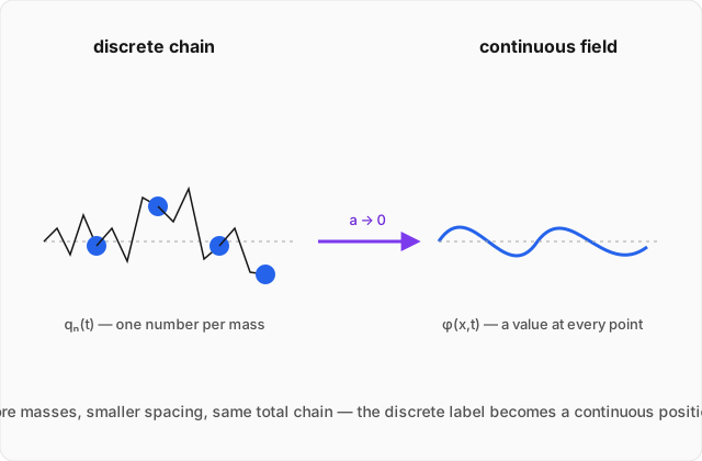
Now make the construction finer. Replace each mass by a smaller one, shorten every spring, and reduce the spacing $a$ , while keeping the total length fixed. As $N\to\infty$ and $a\to 0$ , there is no longer a useful answer to "which mass?" Instead, we ask "at which position?" The discrete label $n$ is replaced by the continuous coordinate

x = na,

and the displacement becomes

q_n(t) \longrightarrow \phi(x,t).

Neighboring displacements differ by

q_{n+1}(t)-q_n(t) = \phi(x+a,t)-\phi(x,t) \approx a\frac{\partial\phi}{\partial x},

while a sum over masses becomes an integral over position:

\sum_n a \longrightarrow \int dx.

This is not a formal trick performed after the physics is finished. It is a physical limiting process: more masses, smaller spacing, the same total object. A field is what mechanics becomes when the system has a degree of freedom at every point in space.

A chain of masses connected by springs on the left, with an arrow showing the continuum limit as the spacing shrinks to zero, producing a smooth continuous field on the right.

The individual displacements of a finer and finer chain merge into one smooth function, turning a discrete list of coordinates, one per bead, into a continuous field with a value at every point of space and time.

What is a field?

A field is a number, or a set of numbers, assigned to every point of space at every time. For a one-dimensional vibrating string, $\phi(x,t)$ might be the vertical displacement of the string at position $x$ and time $t$ . In three dimensions, a field could depend on $(x,y,z,t)$ instead.

You have already met fields informally. A weather map assigns a temperature to every location. The surface of water assigns a height to every horizontal position. But classical field theory asks a more demanding question: if the entire field is a dynamical system, what law determines how its value at every point changes with time?

In ordinary Lagrangian mechanics, a trajectory $q(t)$ is the object whose motion we solve for. In field theory, that object is replaced by a function $\phi(x,t)$ . The field itself is the generalized coordinate, except that there is one coordinate value for every $x$ .

The Lagrangian density

For finitely many coordinates, the Lagrangian is a function such as $L(q_i,\dot q_i,t)$ . For a field spread through space, different regions contribute to the total kinetic and potential energy. The natural local object is therefore a Lagrangian density $\mathcal{L}$ , defined so that

L = \int \mathcal{L}\,dx.

The density may depend on the field, its time derivative, its spatial derivative, and possibly position and time explicitly:

\mathcal{L} = \mathcal{L}\left(\phi,\partial_t\phi,\partial_x\phi,x,t\right).

The action is the time integral of the Lagrangian, so for a field it becomes an integral over both space and time:

S = \int L\,dt = \int\!\int \mathcal{L}\,dx\,dt.

Why work with a density? Because the Lagrangian of the whole field is assembled by adding the contribution from every small interval of space. If an interval $dx$ contributes $\mathcal{L}\,dx$ , then $\mathcal{L}$ is the local quantity from which the global dynamics is built.

The Euler-Lagrange equation for a field

For one coordinate $q(t)$ , stationarity of the action gives the familiar Euler-Lagrange equation

\frac{d}{dt}\left(\frac{\partial L}{\partial\dot q}\right) - \frac{\partial L}{\partial q} = 0.

A field can vary in time and from one spatial point to the next. The variational calculation must therefore account for derivatives in all of those directions. The result is

\partial_\mu\left(\frac{\partial \mathcal{L}}{\partial(\partial_\mu \phi)}\right) - \frac{\partial \mathcal{L}}{\partial \phi} = 0.

The index $\mu$ labels spacetime directions. In one space dimension, it runs over time and $x$ , so the compact equation means

\frac{\partial}{\partial t} \left(\frac{\partial\mathcal{L}}{\partial(\partial_t\phi)}\right) + \frac{\partial}{\partial x} \left(\frac{\partial\mathcal{L}}{\partial(\partial_x\phi)}\right) - \frac{\partial\mathcal{L}}{\partial\phi} =0.

In three space dimensions, $\mu$ runs over $t,x,y,z$ , and there is one derivative term for each direction. The generalization from particle mechanics is now visible: where the particle equation had only the time-derivative term involving $\dot q$ , the field equation has a time-derivative term involving $\partial_t\phi$ and spatial-derivative terms involving $\partial_x\phi$ , $\partial_y\phi$ , and $\partial_z\phi$ .

The spatial term is precisely what lets neighboring points influence one another. Without it, every point would evolve as an isolated mechanical system, unaware that a disturbance had occurred next door.

Worked example

A free scalar field in one spatial dimension has Lagrangian density $\mathcal{L}=\frac{1}{2}(\partial_t\phi)^2-\frac{1}{2}v^2(\partial_x\phi)^2$ . Derive its equation of motion and verify a traveling cosine solution. (click to reveal the solution)

Setting up: the field Euler-Lagrange equation in one space dimension is

\frac{\partial}{\partial t} \left(\frac{\partial\mathcal{L}}{\partial(\partial_t\phi)}\right) + \frac{\partial}{\partial x} \left(\frac{\partial\mathcal{L}}{\partial(\partial_x\phi)}\right) - \frac{\partial\mathcal{L}}{\partial\phi} =0.

For

\mathcal{L} = \frac{1}{2}(\partial_t\phi)^2 - \frac{1}{2}v^2(\partial_x\phi)^2,

we evaluate its three required partial derivatives one at a time.

Derivative with respect to the time derivative of the field:

\frac{\partial\mathcal{L}}{\partial(\partial_t\phi)} = \frac{\partial}{\partial(\partial_t\phi)} \left[\frac{1}{2}(\partial_t\phi)^2 -\frac{1}{2}v^2(\partial_x\phi)^2\right] = \partial_t\phi.

Taking its time derivative gives

\frac{\partial}{\partial t} \left(\frac{\partial\mathcal{L}}{\partial(\partial_t\phi)}\right) = \frac{\partial}{\partial t}(\partial_t\phi) = \partial_t^2\phi.

Derivative with respect to the spatial derivative of the field:

\frac{\partial\mathcal{L}}{\partial(\partial_x\phi)} = \frac{\partial}{\partial(\partial_x\phi)} \left[\frac{1}{2}(\partial_t\phi)^2 -\frac{1}{2}v^2(\partial_x\phi)^2\right] = -v^2\partial_x\phi.

Taking its spatial derivative gives

\frac{\partial}{\partial x} \left(\frac{\partial\mathcal{L}}{\partial(\partial_x\phi)}\right) = \frac{\partial}{\partial x}(-v^2\partial_x\phi) = -v^2\partial_x^2\phi,

where $v$ is constant.

Derivative with respect to the field itself: the density contains derivatives of $\phi$ , but no undifferentiated $\phi$ . Therefore

\frac{\partial\mathcal{L}}{\partial\phi}=0.

Substituting all three results into the Euler-Lagrange equation,

\partial_t^2\phi - v^2\partial_x^2\phi - 0 = 0.

Hence

\boxed{\partial_t^2\phi = v^2\partial_x^2\phi},

which is the wave equation. The constant $v$ has the dimensions of speed and is the propagation speed of disturbances in the field.

Checking a traveling cosine: suppose

\phi(x,t)=A\cos(kx-\omega t).

Its first time derivative is

\partial_t\phi = A\omega\sin(kx-\omega t),

and its second time derivative is

\partial_t^2\phi = -A\omega^2\cos(kx-\omega t).

Its first spatial derivative is

\partial_x\phi = -Ak\sin(kx-\omega t),

and its second spatial derivative is

\partial_x^2\phi = -Ak^2\cos(kx-\omega t).

Substitution into the wave equation gives

-A\omega^2\cos(kx-\omega t) = v^2\left[-Ak^2\cos(kx-\omega t)\right].

For a nonzero wave, the common factor $-A\cos(kx-\omega t)$ cancels, leaving

\omega^2=v^2k^2.

Taking the positive-frequency branch,

\boxed{\omega=vk}.

This is the same move used in simple harmonic motion: guess a cosine, differentiate it twice, and check whether the equation returns the same cosine multiplied by the required constant. For a mass on a spring, the cosine varies only with time. Here it also carries a spatial pattern, and the equation ties that pattern's wavenumber $k$ to its oscillation frequency $\omega$ . The familiar oscillator has not disappeared. It has acquired infinitely many places at which to move.

Where this leads

A general field configuration can be decomposed into independent oscillation modes, much as a complicated musical tone can be decomposed into pure frequencies. For the free field, each mode has its own amplitude and oscillates with its own frequency. Mathematically, the field is therefore an infinite collection of independent harmonic oscillators, one for each allowed mode.

The reader who knows the quantum harmonic oscillator has already seen what quantum mechanics does to one such oscillator: its energy comes in an evenly spaced ladder, and creation and annihilation operators move the system up and down that ladder. Quantizing a field means applying that construction to every mode at once.

One rung up the ladder of a particular field mode is what physics calls a particle. The particle is not an extra object placed into the field; it is a quantum of the field's oscillation. That is the central move of quantum field theory, and classical field theory is the half developed here: the mechanics of the continuous system before its infinitely many oscillators are quantized.