Ordinary Differential Equations

This entire site has been solving differential equations almost from its first page, without stopping to name the general subject. Newton's laws gave us $F=ma$ , which becomes a differential equation whenever the force depends on position, velocity, or time. The equation of simple harmonic motion,

m\ddot x=-kx,

is a differential equation. The pendulum equation is one too. So is the Schrödinger equation.

Yet in each first encounter, we took a suspiciously fortunate route: guess a function, often a cosine, differentiate it, substitute it into the equation, and discover that it works. That proves the guessed function is a solution, but it leaves an uncomfortable question. Where did the guess come from? If the answer were not a cosine, how would we know what to try?

That is the problem ordinary differential equations are meant to organize. An ordinary differential equation, or ODE, relates an unknown function of one independent variable to one or more of its derivatives. The aim is not to eliminate insight or cleverness. It is to replace a collection of lucky guesses with methods that tell us what forms the solutions must take.

Classifying an ODE

Before solving a differential equation, it helps to know what kind of object is in front of us. Three distinctions determine which methods are available.

Order

The order of a differential equation is the order of the highest derivative appearing in it. For example,

\frac{dy}{dx}+3y=0

is first-order, while

m\ddot x+kx=0

is second-order because $\ddot x=d^2x/dt^2$ is the highest derivative present.

The order also tells us how much initial information is generally needed to select one solution from the family of possible solutions. A first-order equation usually requires one initial condition, such as $y(0)$ . A second-order equation usually requires two, such as the initial position $x(0)$ and initial velocity $\dot x(0)$ .

Linear and nonlinear

An ODE is linear if the unknown function and its derivatives appear only to the first power, are not multiplied by one another, and have coefficients that depend at most on the independent variable. A general second-order linear ODE has the form

a_2(t)\ddot y+a_1(t)\dot y+a_0(t)y=g(t).

The equation

m\ddot x+kx=0

is linear. By contrast,

\ddot\theta+\frac{g}{L}\sin\theta=0

for an exact pendulum is nonlinear because $\sin\theta$ is not a linear function of the unknown angle $\theta$ . The small-angle approximation $\sin\theta\approx\theta$ turns it into a linear equation, which is precisely why the approximated pendulum becomes so much easier to solve.

Homogeneous and inhomogeneous

A linear ODE is homogeneous if every term contains the unknown function or one of its derivatives. Thus the simple-harmonic-motion equation

m\ddot x+kx=0

is second-order, linear, and homogeneous.

A linear ODE is inhomogeneous if a leftover term does not contain the unknown function. A driven oscillator obeys

m\ddot x+kx=F(t),

where the prescribed external force $F(t)$ makes the equation inhomogeneous. Physically, this distinction separates the system's free motion from its response to an external drive.

First-order linear equations

Consider the general first-order linear ODE

\frac{dy}{dx}+P(x)y=Q(x).

The difficulty is that the left side is almost, but not quite, the derivative of a product. We would like to multiply the equation by some function $\mu(x)$ so that

\mu(x)\frac{dy}{dx}+\mu(x)P(x)y

becomes one exact derivative. The product rule says

\frac{d}{dx}\left[\mu(x)y(x)\right] =\mu(x)\frac{dy}{dx}+\frac{d\mu}{dx}y.

The two expressions agree if

\frac{d\mu}{dx}=P(x)\mu(x).

Dividing by $\mu$ and integrating,

\frac{1}{\mu}\frac{d\mu}{dx}=P(x),

\int\frac{1}{\mu}\,d\mu=\int P(x)\,dx,

\ln|\mu|=\int P(x)\,dx.

An overall nonzero constant multiplying $\mu$ makes no difference, so we choose the integrating factor

\mu(x)=e^{\int P(x)\,dx}.

Multiplying the original ODE by this factor gives

\mu\frac{dy}{dx}+\mu Py=\mu Q.

Because $d\mu/dx=P\mu$ , the left side is exactly

\frac{d}{dx}(\mu y)=\mu Q.

Now integrate both sides:

\mu(x)y(x)=\int \mu(x)Q(x)\,dx+C,

and therefore

y(x)=\frac{1}{\mu(x)}\left[\int \mu(x)Q(x)\,dx+C\right].

The integrating factor was engineered to make the product rule do the work for us.

Example: solving $y'+2y=e^{-x}$

Start with

\frac{dy}{dx}+2y=e^{-x}.

Here

P(x)=2, \qquad Q(x)=e^{-x}.

The integrating factor is

\mu(x)=e^{\int 2\,dx}=e^{2x}.

Multiply every term in the equation by $e^{2x}$ :

e^{2x}\frac{dy}{dx}+2e^{2x}y=e^{2x}e^{-x}.

The right side simplifies to $e^x$ , while the left side is an exact derivative:

\frac{d}{dx}\left(e^{2x}y\right)=e^x.

Integrating,

e^{2x}y=\int e^x\,dx=e^x+C.

Finally, divide by $e^{2x}$ :

y=e^{-x}+Ce^{-2x}.

We can verify the result directly. Differentiating gives

\frac{dy}{dx}=-e^{-x}-2Ce^{-2x}.

Then

\frac{dy}{dx}+2y =-e^{-x}-2Ce^{-2x}+2e^{-x}+2Ce^{-2x} =e^{-x},

as required. The term $e^{-x}$ is a particular response to the inhomogeneous term, while $Ce^{-2x}$ is the general solution of the corresponding homogeneous equation $y'+2y=0$ .

Second-order equations with constant coefficients

Now consider a second-order linear homogeneous ODE with constant coefficients:

a\ddot y+b\dot y+cy=0,

where $a$ , $b$ , and $c$ are constants and $a\neq0$ .

Here the exponential function has a remarkable property: differentiating it does not produce a new kind of function. If

y=e^{rt},

then

\dot y=re^{rt}

and

\ddot y=r^2e^{rt}.

Substitute these into the differential equation:

ar^2e^{rt}+bre^{rt}+ce^{rt}=0.

Factor out $e^{rt}$ :

e^{rt}(ar^2+br+c)=0.

Since $e^{rt}$ is never zero, the remaining factor must vanish:

ar^2+br+c=0.

This is the characteristic equation. A problem involving derivatives has become an algebraic problem involving a quadratic polynomial.

Its roots are

r=\frac{-b\pm\sqrt{b^2-4ac}}{2a}.

The discriminant

\Delta=b^2-4ac

separates the solutions into three qualitatively different cases.

Two distinct real roots

If $\Delta>0$ , the characteristic equation has two distinct real roots $r_1$ and $r_2$ . The corresponding exponentials are linearly independent, so the general solution is

y(t)=C_1e^{r_1t}+C_2e^{r_2t}.

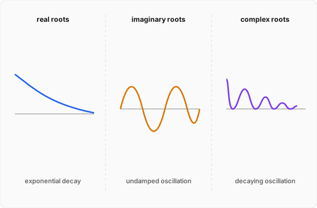
Positive roots produce exponential growth; negative roots produce exponential decay. When both roots are negative, a displaced system can return to equilibrium without crossing it repeatedly.

One repeated real root

If $\Delta=0$ , both roots merge into

r=-\frac{b}{2a}.

The function $e^{rt}$ is one solution, but simply writing it twice does not produce two independent solutions. A second-order equation needs two independent solutions, and the second one is

te^{rt}.

Thus the general solution is

y(t)=(C_1+C_2t)e^{rt}.

One way to understand the factor of $t$ is to imagine two distinct exponential solutions as their roots approach one another. Their difference, divided by the shrinking separation of the roots, approaches a derivative with respect to $r$ :

\frac{\partial}{\partial r}e^{rt}=te^{rt}.

When the two roots merge, this limiting procedure supplies the missing independent solution.

Complex conjugate roots

If $\Delta<0$ , the roots come as a complex conjugate pair

r=\alpha\pm i\beta.

The exponential solutions are

e^{(\alpha+i\beta)t} \qquad\text{and}\qquad e^{(\alpha-i\beta)t}.

Euler's formula,

e^{i\beta t}=\cos(\beta t)+i\sin(\beta t),

lets us combine these into two real solutions:

e^{\alpha t}\cos(\beta t) \qquad\text{and}\qquad e^{\alpha t}\sin(\beta t).

Therefore the general real solution is

y(t)=e^{\alpha t}\left[C_1\cos(\beta t)+C_2\sin(\beta t)\right].

The imaginary part of the root produces oscillation. The real part controls the envelope: $\alpha<0$ gives a decaying oscillation, $\alpha=0$ gives an undamped oscillation, and $\alpha>0$ gives a growing oscillation.

Three small graphs side by side showing the three qualitatively different behaviors of a second-order linear ODE solution: pure exponential growth or decay for real roots, oscillation for purely imaginary roots, and a decaying oscillation (spiral) for complex roots with a negative real part. — The roots of one quadratic decide the motion: real roots give exponential behavior, imaginary roots give oscillation, and complex roots combine an exponential envelope with an oscillation.

Why the cosine appears in simple harmonic motion

For simple harmonic motion, the equation is

m\ddot x+kx=0.

Comparing it with

a\ddot y+b\dot y+cy=0,

we identify

a=m, \qquad b=0, \qquad c=k.

The characteristic equation is

mr^2+k=0.

Therefore

r^2=-\frac{k}{m},

and the roots are

r=\pm i\sqrt{\frac{k}{m}}.

Defining

\omega=\sqrt{\frac{k}{m}},

we have

r=\pm i\omega.

These purely imaginary roots produce the real general solution

x(t)=C_1\cos(\omega t)+C_2\sin(\omega t).

Equivalently, the constants can be repackaged as an amplitude and phase:

x(t)=A\cos(\omega t+\phi).

This is the rigorous reason the cosine guess used on the simple-harmonic-motion page worked. It was not luck. For this particular differential equation, the characteristic roots are necessarily imaginary, and Euler's formula necessarily turns their exponentials into sines and cosines.

Worked example

A damped harmonic oscillator obeys $m\ddot x+b\dot x+kx=0$ . Solve the equation for $m=1\text{ kg}$ , $b=4\text{ kg/s}$ , and $k=3\text{ N/m}$ , then interpret the resulting motion. (click to reveal the solution)

Substituting the parameters: begin with

m\ddot x+b\dot x+kx=0.

Using $m=1$ , $b=4$ , and $k=3$ gives

\ddot x+4\dot x+3x=0.

Setting up the characteristic equation: try

x=e^{rt}.

Then

\dot x=re^{rt}

and

\ddot x=r^2e^{rt}.

Substitution gives

r^2e^{rt}+4re^{rt}+3e^{rt}=0.

Factor out the nonzero exponential:

e^{rt}(r^2+4r+3)=0.

Therefore the characteristic equation is

r^2+4r+3=0.

Finding the roots: factor the quadratic:

r^2+4r+3=(r+1)(r+3).

Thus

(r+1)(r+3)=0,

so the two distinct roots are

r_1=-1\text{ s}^{-1}, \qquad r_2=-3\text{ s}^{-1}.

The same result follows from the quadratic formula:

r=\frac{-4\pm\sqrt{4^2-4(1)(3)}}{2(1)} =\frac{-4\pm\sqrt{16-12}}{2} =\frac{-4\pm2}{2},

which gives $r=-1\text{ s}^{-1}$ and $r=-3\text{ s}^{-1}$ .

Writing the general solution: because the roots are distinct and real,

x(t)=C_1e^{-t}+C_2e^{-3t}.

The constants $C_1$ and $C_2$ would be fixed by two initial conditions, such as $x(0)$ and $\dot x(0)$ .

Physical interpretation: both exponential terms decay as time increases. Neither term contains a sine or cosine, so no oscillation occurs. The damping is strong enough to prevent the mass from swinging repeatedly through equilibrium; instead, the displacement relaxes back toward

\lim_{t\to\infty}x(t)=0.

This is an overdamped oscillator. Its two decay rates describe a rapidly disappearing transient $e^{-3t}$ and a more slowly decaying tail $e^{-t}$ . After enough time, the slower term dominates unless its coefficient happens to be zero.

Where this leads

The move that solved the constant-coefficient equation was to choose functions that reproduce themselves under differentiation. The guess $e^{rt}$ turned a differential equation into an algebraic equation because derivatives act on exponentials only by multiplying them by powers of $r$ .

That idea extends far beyond the equations on this page. Fourier analysis, the next topic in this track, decomposes complicated functions into sums of the same exponential and oscillatory building blocks found here. Later, partial differential equations such as the wave equation and the Schrödinger equation in three dimensions can be attacked by separation of variables, which breaks one equation involving several variables into ordinary differential equations of exactly this kind.