Fourier Analysis and the Fourier Transform

Pluck a guitar string and something strange is happening in the air that reaches your ear. A tuning fork produces something close to a single pure tone: one frequency, one clean sine wave pushing the air back and forth. A plucked string does not. Look at the actual waveform on an oscilloscope and it is a jagged, lopsided, thoroughly complicated shape, repeating once per period of the note but otherwise looking nothing like a sine wave. And yet your ear, and a spectrum analyzer, both report the same fact: buried inside that complicated repeating shape is the fundamental pitch you hear, plus a specific, discrete set of higher overtones, each at its own volume. Somehow a complicated periodic shape is secretly a sum of simple ones.

That "somehow" is not a vague acoustic fact. It is an exact mathematical statement, and classical field theory already told you where it was heading, in a sentence dropped without proof: "a general field configuration can be decomposed into independent oscillation modes, much as a complicated musical tone can be decomposed into pure frequencies." This topic makes that decomposition precise. It is not a special trick invented for waveforms. It is a direct consequence of ideas already sitting in linear algebra, applied to a vector space you have not yet thought to look at that way: the space of functions itself.

Functions as vectors, integrals as dot products

Recall the central move of that earlier topic: strip an object down to nothing but its rules for addition and scalar multiplication, and many unrelated-looking things turn out to be vectors in disguise — arrows, quadratic polynomials, whatever obeys the ten vector-space axioms. Periodic functions qualify immediately. If $f(x)$ and $g(x)$ are both periodic with period $2L$ , so is $af(x)+bg(x)$ for any scalars $a,b$ . The set of such functions is closed under linear combination, exactly like $\mathbb{R}^3$ or the polynomial space $P_2$ from that topic.

But $\mathbb{R}^3$ carried more structure than the bare vector-space axioms supply: a dot product, letting you ask how much of one vector lies along another, and a notion of length and orthogonality built out of it. Functions can carry that structure too. Define, for functions on an interval $[-L,L]$ ,

\langle f,g\rangle \equiv \int_{-L}^{L} f(x)\,g(x)\,dx.

This plays exactly the role of the dot product. Where $\vec u\cdot\vec v=\sum_i u_iv_i$ adds up products of components, $\langle f,g\rangle$ adds up — via an integral instead of a sum — products of function values at every point of the interval. It has the properties a dot product needs: it is linear in each argument, symmetric under $f\leftrightarrow g$ , and $\langle f,f\rangle=\int_{-L}^{L}f(x)^2\,dx\geq0$ , vanishing only if $f$ is zero everywhere on the interval. Two functions are orthogonal when $\langle f,g\rangle=0$ , in precise analogy with $\vec u\cdot\vec v=0$ .

Orthogonality of the trigonometric functions

Here is the fact that makes the whole subject work: the infinite family

\left\{1,\ \cos\frac{\pi x}{L},\ \cos\frac{2\pi x}{L},\ \ldots,\ \sin\frac{\pi x}{L},\ \sin\frac{2\pi x}{L},\ \ldots\right\}

is mutually orthogonal under $\langle\cdot,\cdot\rangle$ on $[-L,L]$ . This is not asserted; it follows directly from the product-to-sum identities. Take two positive integers $n,m$ and use

\cos A\cos B=\tfrac12\left[\cos(A-B)+\cos(A+B)\right]

with $A=n\pi x/L$ , $B=m\pi x/L$ :

\cos\frac{n\pi x}{L}\cos\frac{m\pi x}{L} =\frac12\left[\cos\frac{(n-m)\pi x}{L}+\cos\frac{(n+m)\pi x}{L}\right].

For any nonzero integer $k$ ,

\int_{-L}^{L}\cos\frac{k\pi x}{L}\,dx =\left[\frac{L}{k\pi}\sin\frac{k\pi x}{L}\right]_{-L}^{L} =\frac{L}{k\pi}\left[\sin(k\pi)-\sin(-k\pi)\right]=0,

since $\sin$ vanishes at every integer multiple of $\pi$ ; and for $k=0$ , $\int_{-L}^{L}1\,dx=2L$ . If $n\neq m$ , both $n-m$ and $n+m$ are nonzero, so both terms in the identity integrate to zero:

\int_{-L}^{L}\cos\frac{n\pi x}{L}\cos\frac{m\pi x}{L}\,dx=0,\qquad n\neq m.

If $n=m$ , the first term has $k=0$ and contributes $\tfrac12(2L)=L$ , while the second term still has $k=2n\neq0$ and vanishes. So

\int_{-L}^{L}\cos\frac{n\pi x}{L}\cos\frac{n\pi x}{L}\,dx=L.

The same argument with $\sin A\sin B=\tfrac12\left[\cos(A-B)-\cos(A+B)\right]$ gives $\int_{-L}^{L}\sin(n\pi x/L)\sin(m\pi x/L)\,dx=0$ for $n\neq m$ and $L$ for $n=m$ . Finally, $\sin A\cos B=\tfrac12\left[\sin(A+B)+\sin(A-B)\right]$ , and $\int_{-L}^{L}\sin(k\pi x/L)\,dx=0$ for every integer $k$ (its antiderivative $-\frac{L}{k\pi}\cos(k\pi x/L)$ returns the same, even, cosine value at both endpoints, so the bracket cancels). So every sine is orthogonal to every cosine, with no exception at $n=m$ :

\int_{-L}^{L}\sin\frac{n\pi x}{L}\cos\frac{m\pi x}{L}\,dx=0\quad\text{for all }n,m.

This entire family behaves exactly like the mutually perpendicular basis vectors $\hat x,\hat y,\hat z$ of ordinary space — an orthogonal basis, only for an infinite-dimensional space of functions instead of three-dimensional $\mathbb{R}^3$ .

The coefficient formulas

Suppose a periodic function $f(x)$ can be written as a combination of these basis functions:

f(x)=\frac{a_0}{2}+\sum_{n=1}^{\infty}\left[a_n\cos\frac{n\pi x}{L}+b_n\sin\frac{n\pi x}{L}\right].

In finite dimensions, linear algebra found the coordinates of a vector in a basis just by matching components. Here there are infinitely many unknowns $a_n,b_n$ at once, and matching components directly is hopeless. Orthogonality is what rescues the problem: it lets every coefficient be isolated one at a time, without ever solving a system of equations.

Take the inner product of both sides with $\cos(m\pi x/L)$ for some fixed $m\geq1$ :

\left\langle f,\cos\frac{m\pi x}{L}\right\rangle =\frac{a_0}{2}\left\langle1,\cos\frac{m\pi x}{L}\right\rangle +\sum_{n=1}^{\infty}a_n\left\langle\cos\frac{n\pi x}{L},\cos\frac{m\pi x}{L}\right\rangle +\sum_{n=1}^{\infty}b_n\left\langle\sin\frac{n\pi x}{L},\cos\frac{m\pi x}{L}\right\rangle.

By the orthogonality just derived, every term on the right vanishes except the single term $n=m$ in the cosine sum, which equals $a_mL$ :

\left\langle f,\cos\frac{m\pi x}{L}\right\rangle=a_mL \quad\Longrightarrow\quad a_m=\frac{1}{L}\int_{-L}^{L}f(x)\cos\frac{m\pi x}{L}\,dx.

The identical argument with $\sin(m\pi x/L)$ isolates

b_m=\frac{1}{L}\int_{-L}^{L}f(x)\sin\frac{m\pi x}{L}\,dx,

and taking the inner product with the constant function $1$ gives $a_0=\frac1L\int_{-L}^{L}f(x)\,dx$ , the average value of $f$ over one period (times two, to match the $a_0/2$ convention above). Every Fourier coefficient is a projection: multiply $f$ by a basis function, integrate, divide by the basis function's own squared length $L$ — the exact continuum analogue of $v_i=\vec v\cdot\hat e_i$ for an orthonormal basis of ordinary vectors.

Three panels showing successive approximations to a square wave built from sine harmonics: the first harmonic alone, the sum of the first three odd harmonics, and the sum of many odd harmonics, the last one showing a persistent overshoot near the jump. — Adding more odd harmonics of a square wave brings the partial sum closer to a jagged step everywhere except right at the jump, where a stubborn overshoot survives no matter how many terms are added — the Gibbs phenomenon.

The complex exponential form, and where $e^{rt}$ comes back

Ordinary differential equations built its entire theory of constant-coefficient equations on one observation: the exponential $e^{rt}$ reproduces itself under differentiation, so guessing it turns a differential equation into an algebraic one. When the characteristic roots came out purely imaginary, $r=\pm i\omega$ , Euler's formula converted the complex exponential solutions into the real $\cos(\omega t)$ and $\sin(\omega t)$ pair. Fourier series are built from exactly those same purely-imaginary-root building blocks, just relabeled as functions of position rather than time.

Using Euler's formula in reverse,

\cos\frac{n\pi x}{L}=\frac{e^{in\pi x/L}+e^{-in\pi x/L}}{2}, \qquad \sin\frac{n\pi x}{L}=\frac{e^{in\pi x/L}-e^{-in\pi x/L}}{2i},

substitute these into the real Fourier series and collect terms by exponential. Every $\cos(n\pi x/L)$ and $\sin(n\pi x/L)$ pair, for $n=1,2,3,\ldots$ , contributes to both $e^{in\pi x/L}$ and $e^{-in\pi x/L}$ , and allowing the index to run over all integers (positive, negative, and zero) absorbs the whole series into one sum:

f(x)=\sum_{n=-\infty}^{\infty}c_ne^{in\pi x/L}, \qquad c_n=\frac{1}{2L}\int_{-L}^{L}f(x)\,e^{-in\pi x/L}\,dx.

The relation between $c_n$ and $a_n,b_n$ follows directly from matching the two forms; it is bookkeeping, not new physics. What is worth pausing on is why $e^{in\pi x/L}$ is the natural building block at all: it is the general solution of the same equation type solved on the ordinary-differential-equations page, $y''=-(n\pi/L)^2y$ , whose characteristic roots are $r=\pm in\pi/L$ — purely imaginary, for exactly the same structural reason a frictionless spring's roots were purely imaginary. Each Fourier mode is, secretly, a tiny undamped harmonic oscillator indexed by $n$ .

From series to transform: letting the period run off to infinity

A Fourier series only makes sense for a function that repeats. But most functions worth analyzing in physics — a single pulse, a wave packet, a particle's position probability — do not repeat at all. What happens to the machinery above if the period $2L$ is allowed to grow without bound?

Define $k_n=n\pi/L$ and $\Delta k=\pi/L$ , the spacing between adjacent allowed frequencies. Then $\Delta k/(2\pi)=1/(2L)$ , so the coefficient formula can be rewritten as

c_n=\frac{\Delta k}{2\pi}\int_{-L}^{L}f(x')\,e^{-ik_nx'}\,dx',

and the series becomes

f(x)=\sum_{n=-\infty}^{\infty}c_ne^{ik_nx} =\sum_{n=-\infty}^{\infty}\frac{\Delta k}{2\pi}\left[\int_{-L}^{L}f(x')\,e^{-ik_nx'}\,dx'\right]e^{ik_nx}.

As $L\to\infty$ , two things happen at once: the frequency spacing $\Delta k=\pi/L\to0$ , so the discrete frequencies $k_n$ crowd into a continuum, and the sum over $n$ becomes a Riemann sum in $k$ , turning into an integral:

f(x)=\frac{1}{2\pi}\int_{-\infty}^{\infty}\left[\int_{-\infty}^{\infty}f(x')\,e^{-ikx'}\,dx'\right]e^{ikx}\,dk =\frac{1}{2\pi}\int_{-\infty}^{\infty}F(k)\,e^{ikx}\,dk,

where

F(k)\equiv\int_{-\infty}^{\infty}f(x)\,e^{-ikx}\,dx

is the Fourier transform of $f$ . Nothing about the underlying idea changed: $F(k)$ still measures how much of frequency $k$ is present in $f$ , exactly as $c_n$ measured how much of frequency $k_n$ was present in a periodic function. The only difference is that a function without a period has, in principle, every frequency present by some amount, so the discrete list of coefficients becomes a continuous density.

Worked example

Find the Fourier sine series of the square wave $f(x)=+1$ for $0<x<\pi$ and $f(x)=-1$ for $-\pi<x<0$ , periodic with period $2\pi$ , and describe what happens near the jump as more terms are kept. (click to reveal the solution)

Setting up: this $f$ is an odd function, $f(-x)=-f(x)$ . For an odd $f$ , every cosine coefficient vanishes: $f(x)\cos(nx)$ is odd (odd times even), and the integral of an odd function over the symmetric interval $[-\pi,\pi]$ is zero. So $a_0=0$ and $a_n=0$ for all $n\geq1$ , and only the sine terms survive (here $L=\pi$ , so the basis functions are $\sin(nx)$ ).

Computing $b_n$ : the general formula is

b_n=\frac{1}{\pi}\int_{-\pi}^{\pi}f(x)\sin(nx)\,dx.

Since $f(x)\sin(nx)$ is even (odd times odd), the integral over $[-\pi,\pi]$ is twice the integral over $[0,\pi]$ , where $f(x)=1$ :

b_n=\frac{2}{\pi}\int_{0}^{\pi}\sin(nx)\,dx.

Evaluating the integral,

\int_{0}^{\pi}\sin(nx)\,dx =\left[-\frac{\cos(nx)}{n}\right]_0^{\pi} =-\frac{1}{n}\left[\cos(n\pi)-\cos(0)\right] =\frac{1-\cos(n\pi)}{n}.

Using $\cos(n\pi)=(-1)^n$ ,

b_n=\frac{2}{\pi}\cdot\frac{1-(-1)^n}{n}=\frac{2\left[1-(-1)^n\right]}{n\pi}.

Evaluating for even and odd $n$ : if $n$ is even, $(-1)^n=1$ , so $b_n=0$ . If $n$ is odd, $(-1)^n=-1$ , so

b_n=\frac{2(1-(-1))}{n\pi}=\frac{4}{n\pi}.

Assembling the series: writing $n=2k+1$ for $k=0,1,2,\ldots$ to run over the odd integers only,

\boxed{f(x)=\frac{4}{\pi}\sum_{k=0}^{\infty}\frac{\sin\left[(2k+1)x\right]}{2k+1} =\frac{4}{\pi}\left(\sin x+\frac{\sin 3x}{3}+\frac{\sin 5x}{5}+\cdots\right).}

Only odd harmonics appear, with amplitudes falling off as $1/(2k+1)$ — a slow decay, which is itself a signature of the sharp jump in $f$ : smoother functions have Fourier coefficients that die off faster.

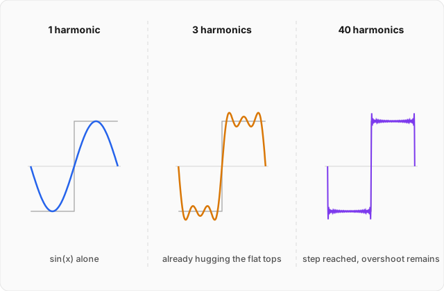
Near the jump: keeping only finitely many terms of this series produces a curve that approximates the square wave increasingly well almost everywhere, wiggling less and hugging the flat tops more tightly as more harmonics are added. But directly next to each jump, at $x=0$ and $x=\pi$ , something does not improve: every partial sum overshoots the top value before turning back down, by very nearly $9\%$ of the total jump height, no matter how many terms are included. Adding more terms squeezes that overshoot into an ever-narrower sliver next to the discontinuity, but its height does not shrink toward zero. This persistent overshoot is the Gibbs phenomenon, a general feature of Fourier approximations to any function with a jump discontinuity, not a peculiarity of this particular square wave. At the jump itself, the series converges to the average of the values on either side, $\frac{(+1)+(-1)}{2}=0$ , exactly the midpoint of the jump.

Where this leads

Fourier series were built on a finite interval, with a discrete, countable family of allowed frequencies $k_n=n\pi/L$ ; the Fourier transform removed the interval and let those frequencies merge into a continuum. Both objects reappear immediately in partial differential equations, the next topic in this track: solving the wave equation on a string of finite length, fixed at both ends, hands back exactly the same sine functions built here, with the coefficients determined by decomposing the string's initial shape into precisely this basis. The square wave solved above will return there as a literal initial condition — a plucked string given that jagged shape at $t=0$ — and the coefficients found here will become the amplitudes of the string's individual vibration modes.