Partial Differential Equations and Separation of Variables

Classical field theory handed you the wave equation,

\partial_t^2\phi=v^2\partial_x^2\phi,

and solved it by guessing a traveling cosine, $\phi(x,t)=A\cos(kx-\omega t)$ , substituting, and checking that it works. Quantum mechanics handed you the Schrödinger equation,

i\hbar\,\partial_t\psi=\hat H\psi,

and solved an important special case by guessing a product form, $\psi(x,t)=\phi(x)T(t)$ , substituting, and discovering that the equation splits cleanly into two independent pieces: one pure function of $t$ , one pure function of $x$ . Both of these were already real results, honestly earned. What went unsaid in both cases is that neither was a coincidence, and they were not two unrelated tricks. They are one method, general enough to tame almost any linear partial differential equation you will meet in physics, and it has a name: separation of variables.

What makes an equation "partial"

Ordinary differential equations relate an unknown function of one variable to its derivatives with respect to that variable. A partial differential equation, or PDE, relates an unknown function of two or more independent variables to its partial derivatives with respect to more than one of them. The wave equation above involves $\partial_t^2\phi$ and $\partial_x^2\phi$ together — the unknown $\phi(x,t)$ genuinely depends on both $x$ and $t$ , and the equation ties their derivatives to one another. That coupling is exactly what makes a PDE harder than an ODE: you cannot simply integrate with respect to $t$ while pretending $x$ is not there, because the equation itself refuses to let $x$ and $t$ go their separate ways — or so it seems, until you try the following.

The method: assume a product, and watch the equation fall apart

Consider a linear PDE for an unknown function $u(x,t)$ . Assume, as a trial solution, that $u$ can be written as a product of a function of $x$ alone and a function of $t$ alone:

u(x,t)=X(x)T(t).

This is a genuine assumption, not a general fact — most solutions of a PDE cannot be written this way. But substitute it into the equation anyway and see what happens. Because $X(x)$ does not depend on $t$ and $T(t)$ does not depend on $x$ , every derivative simplifies: $\partial_t u = X(x)\dot T(t)$ , $\partial_x u = X'(x)T(t)$ , and so on. When the PDE is linear and each term involves derivatives with respect to only one variable at a time (true of the wave equation, the Schrödinger equation, and a great many others), substituting the product form and dividing through by $X(x)T(t)$ separates the equation into two pieces: one side depends only on $x$ , the other only on $t$ . A function of $x$ alone can equal a function of $t$ alone, for every value of both variables, only if both sides equal the same constant — because if you wiggle $t$ while holding $x$ fixed, the left side does not move, so the right side cannot move either. That shared constant is called the separation constant, and it is the single number that couples the two halves of the problem back together. Each half is now an ordinary differential equation, in one variable, solvable with exactly the tools built on that earlier page.

Worked example

A string of length $L$ is fixed at both ends and obeys the wave equation $\partial_t^2\phi=v^2\partial_x^2\phi$ with $\phi(0,t)=\phi(L,t)=0$ . Find its normal modes by separation of variables, and connect the result to the Fourier sine series derived earlier. (click to reveal the solution)

Assuming a product solution: let

\phi(x,t)=X(x)T(t).

Then $\partial_t^2\phi=X(x)\ddot T(t)$ and $\partial_x^2\phi=X''(x)T(t)$ . Substituting into the wave equation,

X(x)\ddot T(t)=v^2X''(x)T(t).

Separating the variables: divide both sides by $X(x)T(t)$ :

\frac{\ddot T(t)}{T(t)}=v^2\frac{X''(x)}{X(x)}.

The left side is a function of $t$ alone; the right side is a function of $x$ alone. Holding $t$ fixed and varying $x$ , the left side cannot change, so the right side must be constant in $x$ too — and by the same argument applied the other way, the left side must be constant in $t$ . Call the shared constant $-\omega^2$ (the choice of sign, and of calling it $\omega^2$ , is a bet that the solution will oscillate rather than blow up — a bet checked and confirmed below):

\frac{\ddot T(t)}{T(t)}=-\omega^2, \qquad v^2\frac{X''(x)}{X(x)}=-\omega^2.

This produces two separate ordinary differential equations:

\ddot T+\omega^2T=0, \qquad X''+k^2X=0, \qquad\text{where}\qquad k\equiv\frac{\omega}{v}.

Solving each ODE: both are the constant-coefficient equation solved on the ordinary differential equations page, with characteristic roots $r=\pm i\omega$ and $r=\pm ik$ respectively — purely imaginary in both cases, giving purely oscillatory solutions:

T(t)=A\cos(\omega t)+B\sin(\omega t), \qquad X(x)=C\sin(kx)+D\cos(kx).

Applying the boundary conditions: the string is nailed down at both ends, so $\phi(0,t)=0$ and $\phi(L,t)=0$ for all $t$ , which force $X(0)=0$ and $X(L)=0$ . From $X(0)=C\sin(0)+D\cos(0)=D=0$ , so $D=0$ and

X(x)=C\sin(kx).

From $X(L)=C\sin(kL)=0$ , and $C=0$ would make $\phi$ vanish everywhere (no motion at all), so instead

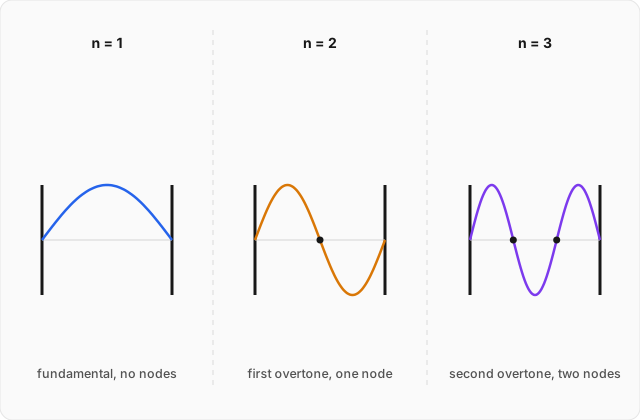
\sin(kL)=0 \quad\Longrightarrow\quad kL=n\pi,\qquad n=1,2,3,\ldots

This is exactly the same boundary-condition arithmetic that forced discrete momenta on the trapped particle in the infinite square well: a function that must vanish at both walls can only fit an integer number of half-wavelengths between them. Here it gives the allowed wavenumbers and frequencies

k_n=\frac{n\pi}{L}, \qquad \omega_n=vk_n=\frac{n\pi v}{L}.

Assembling the normal modes: each allowed $n$ contributes an independent solution $\sin(k_nx)\left[A_n\cos(\omega_nt)+B_n\sin(\omega_nt)\right]$ , and because the wave equation is linear, any sum of these is also a solution. The general vibration of the fixed string is therefore

\phi(x,t)=\sum_{n=1}^{\infty}\sin\!\left(\frac{n\pi x}{L}\right)\left[A_n\cos(\omega_nt)+B_n\sin(\omega_nt)\right].

Connecting to Fourier analysis: the coefficients $A_n$ are fixed by the string's initial shape, $\phi(x,0)=f(x)$ . Setting $t=0$ in the general solution (every $\sin(\omega_n\cdot0)=0$ term drops out) gives

f(x)=\sum_{n=1}^{\infty}A_n\sin\!\left(\frac{n\pi x}{L}\right),

which is exactly a Fourier sine series of the kind derived in Fourier analysis, with $A_n$ given by that page's projection formula, $A_n=\frac{2}{L}\int_0^Lf(x)\sin(n\pi x/L)\,dx$ . If the string were released from a shape resembling the square wave solved there, the amplitudes of its vibration modes would be exactly the coefficients $b_n=4/(n\pi)$ found on that page, one per odd harmonic. The sine functions that made Fourier analysis work are not a mathematical convenience borrowed for this problem — they are the actual normal modes the wave equation forces into existence once you nail down both ends of the string.

Three stacked panels showing a string fixed at both ends vibrating in its first, second, and third normal modes, each with a different number of nodes between the fixed endpoints. — Separation of variables converts one partial differential equation into a family of ordinary ones; the boundary conditions then permit only a discrete ladder of standing-wave shapes, indexed by how many times the string crosses zero between its fixed ends.

The same trick, already used, on the Schrödinger equation

Look back at how quantum mechanics found its stationary states. It assumed $\psi(x,t)=\phi(x)T(t)$ , substituted into $i\hbar\,\partial_t\psi=\hat H\psi$ , and — because $\hat H$ acts only on the $x$ -dependence — obtained

i\hbar\phi(x)\dot T(t)=T(t)\hat H\phi(x).

Dividing both sides by $\phi(x)T(t)$ separates it immediately:

i\hbar\frac{\dot T(t)}{T(t)}=\frac{\hat H\phi(x)}{\phi(x)}.

The left side depends only on $t$ ; the right side, though it involves the operator $\hat H$ , produces a result depending only on $x$ once it acts on $\phi$ . By the identical argument used for the string, both sides must equal the same constant — call it $E$ , and it will turn out to be the energy:

i\hbar\frac{\dot T(t)}{T(t)}=E \quad\Longrightarrow\quad T(t)=e^{-iEt/\hbar},

\hat H\phi(x)=E\phi(x),

which is exactly the time-independent Schrödinger equation from that page. The separation constant is not an abstract bookkeeping device here; it is the one number both halves of the problem must agree on, and demanding that agreement is precisely what turns "the allowed energies" into an eigenvalue problem instead of a guess.

Where this leads

Separation of variables has now been used on a PDE in one spatial dimension plus time. But the Schrödinger equation for a real atom, and Laplace's equation for a gravitational or electric potential around any object that is not perfectly spherical, live in three spatial dimensions with a natural center — spherical symmetry, not a line segment with two endpoints. The next topic, special functions: Legendre polynomials and spherical harmonics, applies exactly this method to that geometry, separating radius from angle, and shows that the angular piece of the separation is where the integer quantum numbers of atomic physics are actually born.