Tensor Calculus: Covariant and Contravariant Indices

Take two objects that both look like ordinary vectors. The first is a tiny displacement, $dx^i$ , an arrow from one nearby point to another. The second is the gradient of some scalar field, $\partial\phi/\partial x^i$ , built in vector calculus as the object whose dot product with a direction gives the rate of change that way. Both have components labeled by an index $i$ running over the coordinate directions. Both were treated, on every page of this site so far, as thoroughly interchangeable — you could dot one against the other, add them, rotate them by the same rotation matrix, and nothing ever went wrong.

Nothing ever went wrong because every calculation on this site so far has stayed inside Cartesian coordinates, related to each other only by rotations. Now change the setup: describe the same plane using polar coordinates instead, or imagine a coordinate grid painted onto a curved surface, where there is no way to lay down a single straight Cartesian grid over the whole thing at all. Ask how $dx^i$ and $\partial\phi/\partial x^i$ transform when you switch from one coordinate system to another, and something that was invisible in Cartesian coordinates suddenly matters enormously: they transform by inverse rules. Treat them as interchangeable in a general coordinate system and you get the wrong physics — a computed force, a computed curvature, an entire computed law that silently depends on which coordinate grid you happened to draw, which is precisely the one thing a real physical law must never do. This matters for more than bookkeeping: general relativity describes gravity as the geometry of a spacetime that is actually curved, with no global Cartesian coordinate patch covering it at all — a story for a later topic, but the reason tensor calculus exists as a subject rather than a footnote to linear algebra.

Two transformation laws, told apart

Let $x^i$ denote a set of coordinates (the superscript is a label, not an exponent — this index-upstairs notation is used everywhere from here on), and let $x'^i$ denote a different coordinate system covering the same space, related to the first by some smooth, invertible map $x'^i=x'^i(x^1,\ldots,x^n)$ . Differentiating that relationship gives the transformation rule for an ordinary displacement:

dx'^i = \sum_j \frac{\partial x'^i}{\partial x^j}\,dx^j.

Any object $V^i$ that transforms this same way under a change of coordinates,

V'^i = \sum_j\frac{\partial x'^i}{\partial x^j}V^j,

is called a contravariant vector. The name is not important; what matters is which Jacobian matrix — $\partial x'^i/\partial x^j$ , built from the new coordinates differentiated with respect to the old — appears in the rule.

Now do the same for the gradient. The chain rule gives, for any scalar field $\phi$ ,

\frac{\partial\phi}{\partial x'^i} = \sum_j\frac{\partial\phi}{\partial x^j}\frac{\partial x^j}{\partial x'^i}.

Any object $\omega_i$ that transforms this way,

\omega'_i = \sum_j\frac{\partial x^j}{\partial x'^i}\,\omega_j,

is called a covariant vector, and is conventionally written with the index downstairs. The Jacobian matrix here — $\partial x^j/\partial x'^i$ , the old coordinates differentiated with respect to the new — is generally a completely different matrix from the one that governed $V^i$ .

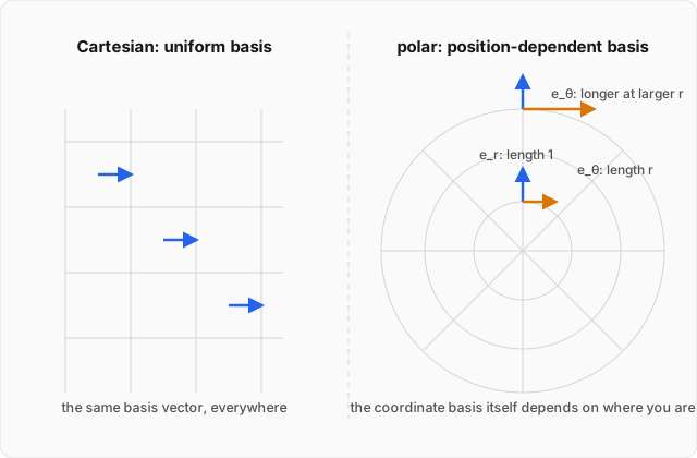
Why did this distinction never matter before? Restrict to Cartesian coordinates related only by a rotation $R$ . The Jacobian matrix $\partial x'^i/\partial x^j$ is then simply the constant matrix $R$ , and — as already shown when linear algebra verified that a rotation matrix satisfies $R^TR=I$ — its inverse equals its own transpose. The two transformation rules above, built from a matrix and from that same matrix's inverse-transpose, become numerically identical for an orthogonal $R$ . Contravariant and covariant components coincide, and the distinction is invisible. Switch to polar coordinates, where the Jacobian varies from point to point and is not even a square rotation of constant vectors, and the two rules genuinely diverge. That divergence is the entire subject of this topic.

Tensors and the Einstein summation convention

A tensor generalizes both of these at once. A tensor of type $(p,q)$ is a multilinear object with $p$ upper (contravariant) indices and $q$ lower (covariant) indices,

T^{i_1\cdots i_p}_{\ \ \ \ \ \ \ j_1\cdots j_q},

transforming under a coordinate change with one factor of $\partial x'^i/\partial x^j$ for every upper index and one factor of $\partial x^j/\partial x'^i$ for every lower index. A scalar is a $(0,0)$ tensor — unchanged by any coordinate transformation, which is exactly what makes a scalar physically meaningful independent of how it's described. A contravariant vector is a $(1,0)$ tensor; a covariant vector is a $(0,1)$ tensor. "Multilinear" means the object is linear separately in each index it carries — feed it one covector and $q-1$ vectors at a time, say, and it responds linearly to each — the direct generalization of the linear maps already built in linear algebra.

Expressions like the ones above are cluttered with summation signs, and one of Einstein's genuine contributions to notation — not just to physics — was to notice that in every sum that actually shows up, the repeated index always appears once upstairs and once downstairs. The Einstein summation convention simply agrees to drop the $\sum$ sign whenever an index is repeated once up and once down in the same expression:

A^iB_i \equiv \sum_i A^iB_i.

From here on, a repeated upper-lower index pair is understood to be summed, and an index that is not repeated is a free index, taking on the same value on both sides of an equation. This is not merely a shorthand; the convention only ever pairs an upper index with a lower one because that is precisely the combination that transforms consistently, as the next section makes explicit.

The metric tensor

Contravariant and covariant vectors both describe "vectors" in some sense, but they are different objects living in different spaces, related by different transformation rules. What converts one into the other? The metric tensor $g_{ij}$ , a $(0,2)$ tensor defined so that the invariant squared distance between two infinitesimally separated points is

ds^2 = g_{ij}\,dx^i\,dx^j.

In ordinary Cartesian coordinates in the plane, $g_{ij}=\delta_{ij}$ (that is, $g_{11}=g_{22}=1,\ g_{12}=g_{21}=0$ ), reproducing the familiar $ds^2=dx^2+dy^2$ . But $g_{ij}$ is defined in any coordinate system, and away from Cartesian coordinates it generally is not the identity — which is exactly the tool the worked example below puts to use.

The metric does more than measure distance: it is the tensor that lowers an index, converting a contravariant vector into its covariant counterpart,

V_i = g_{ij}V^j,

and its matrix inverse $g^{ij}$ (defined by $g^{ij}g_{jk}=\delta^i_k$ , the mixed Kronecker delta, which is $1$ if $i=k$ and $0$ otherwise) raises an index back:

V^i = g^{ij}V_j.

This is the precise machinery that quietly makes "displacement" and "gradient" into a single unified object once a metric is in play, even though they transform by different rules in isolation.

In Cartesian coordinates the basis vectors are the same arrow everywhere. In polar coordinates the radial basis vector stays unit length, but the tangential basis vector grows with the radius — exactly the position-dependence encoded in the angular-angular component of the metric, which equals the radius squared.

Worked example

Derive the metric tensor for polar coordinates $(r,\theta)$ in the plane, find its inverse, verify the contraction $g^{ij}g_{jk}=\delta^i_k$ explicitly, and use the metric to compute the invariant squared speed $g_{ij}\dot x^i\dot x^j$ of a moving particle. (click to reveal the solution)

Setting up: polar coordinates relate to Cartesian coordinates by

x = r\cos\theta, \qquad y = r\sin\theta.

Differentiating,

dx = \cos\theta\,dr - r\sin\theta\,d\theta, \qquad dy = \sin\theta\,dr + r\cos\theta\,d\theta.

Deriving the metric components: substitute into the Cartesian line element $ds^2=dx^2+dy^2$ :

ds^2 = (\cos\theta\,dr - r\sin\theta\,d\theta)^2 + (\sin\theta\,dr + r\cos\theta\,d\theta)^2.

Expanding the first square,

\cos^2\theta\,dr^2 - 2r\sin\theta\cos\theta\,dr\,d\theta + r^2\sin^2\theta\,d\theta^2,

and the second,

\sin^2\theta\,dr^2 + 2r\sin\theta\cos\theta\,dr\,d\theta + r^2\cos^2\theta\,d\theta^2.

The cross terms are equal and opposite, and cancel. Adding what remains,

ds^2 = (\cos^2\theta+\sin^2\theta)\,dr^2 + r^2(\sin^2\theta+\cos^2\theta)\,d\theta^2 = dr^2 + r^2\,d\theta^2.

Comparing with $ds^2=g_{ij}dx^idx^j$ where $(x^1,x^2)=(r,\theta)$ , read off

g_{rr}=1,\qquad g_{\theta\theta}=r^2,\qquad g_{r\theta}=g_{\theta r}=0.

As a matrix,

g_{ij} = \begin{pmatrix}1&0\\0&r^2\end{pmatrix}.

Finding the inverse metric: since $g_{ij}$ is diagonal, its inverse is just the matrix of reciprocals of the diagonal entries:

g^{ij} = \begin{pmatrix}1&0\\0&1/r^2\end{pmatrix}, \qquad\text{that is,}\qquad g^{rr}=1,\qquad g^{\theta\theta}=\frac{1}{r^2},\qquad g^{r\theta}=g^{\theta r}=0.

Verifying the contraction $g^{ij}g_{jk}=\delta^i_k$ explicitly: this is just the statement that the matrices $g^{ij}$ and $g_{jk}$ are inverses of one another, checked directly by matrix multiplication:

g^{ij}g_{jk} = \begin{pmatrix}1&0\\0&1/r^2\end{pmatrix}\begin{pmatrix}1&0\\0&r^2\end{pmatrix} = \begin{pmatrix}1\cdot1+0\cdot0 & 1\cdot0+0\cdot r^2\\ 0\cdot1+\frac{1}{r^2}\cdot0 & 0\cdot0+\frac{1}{r^2}\cdot r^2\end{pmatrix} = \begin{pmatrix}1&0\\0&1\end{pmatrix}.

The result is exactly the identity matrix, whose entries are the mixed Kronecker delta $\delta^i_k$ ( $1$ on the diagonal, $0$ off it). The contraction $g^{ij}g_{jk}=\delta^i_k$ holds, confirming that $g^{ij}$ really is the matrix inverse the raising-and-lowering machinery requires it to be.

Computing the invariant squared speed: a particle moving through the plane has contravariant velocity components $\dot x^i=(\dot r,\dot\theta)$ — the rates of change of the coordinates themselves, which transform exactly like the $dx^i$ that opened this topic. Its invariant squared speed is the scalar built by contracting these components with the metric, $g_{ij}\dot x^i\dot x^j$ . Writing out the sum over both $i$ and $j$ (there are four terms, but the off-diagonal ones vanish since $g_{r\theta}=0$ ):

g_{ij}\dot x^i\dot x^j = g_{rr}\dot r^2 + g_{\theta\theta}\dot\theta^2 = \dot r^2 + r^2\dot\theta^2.

This is exactly the familiar formula for the squared speed of a particle in polar coordinates. It was not derived here from a picture of perpendicular radial and tangential velocity components; it fell directly out of contracting the coordinate velocity with the metric tensor computed above — the same formula, produced by a completely general piece of machinery that works in any coordinate system once you know $g_{ij}$ , not just in the one you happen to already have a geometric picture for.

Where this leads

The metric tensor did more work in that worked example than it may have looked: it converted the bare coordinate velocity $\dot x^i$ , which by itself carries no notion of length at all, into a single physically meaningful number, the speed. That is the entire point of building tensors in the first place — physical quantities like speed, curvature, or energy density must come out the same regardless of which coordinate grid was used to compute them, and a quantity assembled by fully contracting tensor indices (upper against lower, exactly as the summation convention insists) is guaranteed to do exactly that, in any coordinate system whatsoever, curved or flat.

That guarantee is precisely why tensors, and no lesser structure, are the language general relativity is written in: spacetime there is genuinely curved, with no single Cartesian grid covering it globally, so a law of physics had better be built entirely out of objects that transform correctly between any two of its coordinate patches. This topic developed exactly that machinery, in the tamest possible curved-coordinate setting — polar coordinates on a flat plane — as the warm-up act for a much bigger stage still to come.