The Costs of Production

Amara has run the same neighbourhood bakery for six years, and last winter she started keeping a spreadsheet. Every day she wrote down two numbers: how many loaves she baked, and what the whole day cost her — oven lease, insurance, flour, the bakers she called in. Then she divided one by the other to get the cost of an average loaf.

The pattern she found made no sense to her at first. On a quiet Tuesday she baked 40 loaves, and the day cost $500 — $12.50 a loaf. On a frantic Saturday before a holiday she baked 160 loaves, and the day cost $2,000 — again $12.50 a loaf, to the cent. But on an ordinary Thursday she baked 80 loaves for $800, which is $10 a loaf. Two very different days cost the same per loaf, and a day exactly between them was 20% cheaper per loaf than either.

That is a strange shape for a cost to have. Costs are supposed to be costs — you would expect each loaf to cost whatever a loaf costs. Instead the number falls, bottoms out, and climbs back, and the bottom sits at one particular quantity: 80 loaves, not 79 and not 81. Amara's real question, the one that decides whether she should take Saturday orders at all, is where that bottom is and what puts it there.

There is a second reason to care, and it is bigger than one bakery. The supply and demand topic drew an upward-sloping supply curve and justified it with a sentence: at low prices only the cheapest sellers bother, and at higher prices sellers with higher costs find it worthwhile. That sentence was doing an enormous amount of unexamined work. Where do a seller's costs come from? Why should the cost of producing one more unit rise as a firm produces more, which is the only thing that can make a supply curve slope up? The supply curve was asserted. This topic opens it up, and it turns out that everything — the shape of the curve, the bottom of Amara's spreadsheet, the whole apparatus — falls out of one physical fact about production and one line of calculus.

Inside the black box: the production function

Start where cost actually starts, which is not with money at all but with a physical relationship: inputs in, output out. Amara's bakery has one commercial oven, which she leases, and it is the same oven whether she bakes 10 loaves or 200. What she can vary from day to day is labour — how many bakers she calls in. Write $L$ for bakers hired for the day and $q$ for loaves produced. The production function is the rule connecting them, and for this bakery it is

One baker produces 40 loaves in a day. What does the second produce? Not another 40. Two bakers produce $40\sqrt{2} \approx 56.6$ loaves, so the second baker added about 16.6. Tabulate it at the labour levels where the arithmetic is exact — total product $q$, and alongside it the marginal product of labour $MP_L = \dfrac{dq}{dL} = \dfrac{20}{\sqrt{L}}$, the extra output from a marginal extra baker:

The marginal product falls, and it falls fast: the fourth baker's marginal contribution is half the first's, the sixteenth's is a quarter. You can see the same thing without calculus by taking discrete blocks — going from 1 baker to 4 adds 40 loaves for 3 extra workers, about 13.3 loaves each; going from 9 to 16 adds 40 loaves for 7 extra workers, about 5.7 each.

This is diminishing marginal product, and the reason for it in this bakery is not mysterious or moral. It is the oven. One baker has the oven entirely to herself. Four bakers share it: they queue for the racks, they wait on proofing, they get in each other's way at the bench. The oven is fixed, so every extra baker is spread over a thinner slice of the one input that actually bakes bread. Nothing here says the fourth baker is lazier than the first. She is exactly as good — she just has a quarter of an oven to work with.

Hold on to the precise statement, because a later section will contrast it with something that sounds identical and is not: diminishing marginal product is about varying one input while the others are held fixed.

From the production function to the cost curve

Now put prices on the inputs. Amara pays a baker $100 for the day, so $w = 100$. Her fixed costs (the oven lease, insurance, licences, the standby utilities) come to a flat $400 a day whether she bakes or not, so $F = 400$.

To get cost as a function of output, invert the production function: ask not "how much output from $L$ bakers?" but "how many bakers to make $q$ loaves?" From $q = 40\sqrt{L}$,

Total cost is the fixed cost plus the wage bill:

Check it against Amara's spreadsheet immediately, because a cost function you haven't checked is a guess. At $q = 40$: $400 + 1600/16 = 400 + 100 = 500$. ✓ At $q = 80$: $400 + 6400/16 = 400 + 400 = 800$. ✓ At $q = 160$: $400 + 25600/16 = 400 + 1600 = 2000$. ✓ All three of her days.

Notice what the algebra did to the shape. The production function had a square root in it — output grows more slowly than labour. Inverting a square root gives a square — labour, and therefore cost, grows faster than output. The convexity of the cost curve is diminishing marginal product, turned inside out.

That is worth proving in general rather than reading off one example. Let $f$ be any production function with $f' > 0$ (more labour, more output) and $f'' < 0$ (diminishing marginal product). Total cost is $TC(q) = F + w f^{-1}(q)$, and by the inverse function rule $\dfrac{dL}{dq} = \dfrac{1}{f'(L)} = \dfrac{1}{MP_L}$. So marginal cost — the derivative of total cost with respect to output — is

Read that equation slowly, because it is the hinge of the whole topic: the cost of one more loaf is the wage divided by how many loaves a marginal worker-hour produces. If a marginal baker makes 20 loaves and costs $100, the marginal loaf costs $5. If a marginal baker makes only 10 loaves for the same $100, the marginal loaf costs $10. Differentiate once more to get the curvature:

where the middle step used the chain rule, $\dfrac{d\,MP_L}{dq} = \dfrac{d\,MP_L}{dL}\cdot\dfrac{dL}{dq} = \dfrac{f''(L)}{MP_L}$. Since $w > 0$ and $MP_L > 0$, the sign of $dMC/dq$ is the opposite of the sign of $f''$. Diminishing marginal product ($f'' < 0$) therefore forces marginal cost to rise, which forces total cost to be convex. There is no way to have one without the other.

Check the general result against the bakery. Here $f(L) = 40L^{1/2}$, so $f'(L) = 20L^{-1/2} = MP_L$ and $f''(L) = -10L^{-3/2}$. Then

And directly from $TC = 400 + q^2/16$: $MC = q/8$, whose slope is $1/8$. ✓ Same number, by two routes that share no arithmetic.

One more consistency check of the hinge equation itself. At $q = 80$ the bakery uses $L = 80^2/1600 = 4$ bakers, so $MP_L = 20/\sqrt{4} = 10$ and $MC = w/MP_L = 100/10 = 10$ dollars per loaf. From the cost function, $MC = q/8 = 80/8 = 10$. ✓

Six cost concepts, and the algebra tying them together

With $TC(q) = 400 + q^2/16$ in hand, every cost concept in microeconomics is a rearrangement of it. There are six, and they are worth defining precisely once rather than approximately six times.

Fixed cost $FC$ is the part that does not move with output: $FC = 400$. It is the oven lease, and it is $400 whether Amara bakes 200 loaves or closes for the day.

Variable cost $VC(q)$ is the part that does: $VC(q) = q^2/16$, the wage bill. It is zero at zero output.

Total cost is their sum, which is just the definition written out: $TC(q) = FC + VC(q)$.

Average fixed cost $AFC(q) = FC/q = 400/q$ — the overhead, spread over the loaves that carry it. This falls forever, and it never reaches zero. Bakers call it "spreading the oven".

Average variable cost $AVC(q) = VC(q)/q = q/16$.

Average total cost $ATC(q) = TC(q)/q = 400/q + q/16$. This is the number in Amara's spreadsheet. Since $TC = FC + VC$, dividing through by $q$ gives an identity you should be able to see instantly:

Marginal cost $MC(q) = \dfrac{d\,TC}{dq} = \dfrac{q}{8}$, the cost of the next loaf. And here is a small point with large consequences:

because the derivative of a constant is zero. Fixed cost is invisible at the margin. Amara's oven lease does not appear anywhere in the cost of the next loaf; it cannot, because baking that loaf does not change the lease. Every decision about how much more to produce is made entirely with variable costs, which is why "but I have to cover my overheads" is not a reason to bake one more loaf.

Running the other way, marginal cost integrates back to variable cost — not to total cost, since the constant of integration is exactly the fixed cost that fell out:

Here is the whole schedule, in dollars per day and dollars per loaf, with $L = q^2/1600$ shown so you can see the physical side underneath:

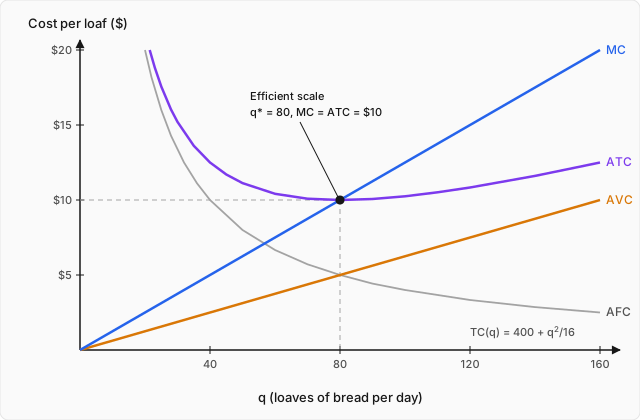
Read the $ATC$ column down: $12.5$, $10.42$, $10$, $10.25$, $10.83$, $12.5$. It falls, bottoms at $q = 80$, and climbs — Amara's spreadsheet, reproduced from a production function and two prices. And now look at the $MC$ column beside it. At $q = 40$, $MC = 5$ while $ATC = 12.5$: marginal cost is below average, and average is falling. At $q = 120$, $MC = 15$ while $ATC = 10.83$: marginal is above average, and average is rising. At $q = 80$ — the bottom — they are equal, both exactly $10$.

That is not a coincidence about this bakery, and it is not a rule of thumb. It is a theorem.

Why marginal cost cuts average cost at its lowest point

Average total cost is total cost divided by quantity, so differentiate exactly that, with the quotient rule and nothing else:

The two terms in the bracket are things we have already named: $TC'(q)$ is marginal cost, and $TC(q)/q$ is average total cost. So

For any positive quantity, $q > 0$, so the sign of the whole expression is the sign of $MC - ATC$. Three statements follow immediately, and they are the entire content of every cost diagram ever drawn:

• If $MC < ATC$, then $ATC' < 0$: average cost is falling.
• If $MC > ATC$, then $ATC' > 0$: average cost is rising.
• $ATC$ is stationary — flat, a candidate minimum — if and only if $MC = ATC$.

The mechanism, once you see it, is almost embarrassing in its simplicity: an average is pulled toward whatever you add to it. Add a loaf costing less than the current average, and the average must fall. Add one costing more, and it must rise. The average can only stop moving at the moment the next item costs exactly what the average already is.

Stationary is not the same as minimum, so finish the job with the second-order condition. Differentiate the boxed identity again:

Evaluate at a stationary point $q_0$, where by construction $ATC'(q_0) = 0$ and $MC(q_0) - ATC(q_0) = 0$. Both of those kill terms, leaving

So the stationary point is a genuine minimum precisely when marginal cost is rising there. Which, from the previous section, is precisely when the firm has diminishing marginal product. The whole chain holds together: diminishing marginal product $\Rightarrow$ marginal cost rising $\Rightarrow$ the point where $MC$ meets $ATC$ is the bottom of $ATC$, and the $MC$ curve cuts the $ATC$ curve there from below.

Verify all of it on the bakery. $ATC(q) = 400/q + q/16$, so

and $ATC(80) = 400/80 + 80/16 = 5 + 5 = 10$, while $MC(80) = 80/8 = 10$. Equal, as the theorem demands. ✓ The boxed identity gives the same derivative independently: $\dfrac{MC - ATC}{q} = \dfrac{1}{q}\left(\dfrac{q}{8} - \dfrac{400}{q} - \dfrac{q}{16}\right) = \dfrac{1}{16} - \dfrac{400}{q^2}$, which is $ATC'$ exactly. ✓ And the second-order check: $ATC''(q) = 800/q^3$, so $ATC''(80) = 800/512000 = 1/640$, while $MC'(q_0)/q_0 = (1/8)/80 = 1/640$. ✓

The quantity $q^* = 80$ has a name: it is the firm's efficient scale, the output at which it produces most cheaply per unit. Notice what it is not: it is not the output that makes the most money. Nothing in this topic has mentioned revenue. Efficient scale is a fact about the cost side alone.

Two smaller observations that the table has already handed you. First, the identical derivation works for average variable cost, since $MC = VC'$ as well:

In this bakery $AVC = q/16$ rises from the very first loaf — $AVC' = 1/16 > 0$ everywhere — so it has no interior minimum, and consistently, $MC - AVC = q/8 - q/16 = q/16$ is positive everywhere: marginal cost sits above average variable cost at every output. The two only meet at the origin, where both are zero. (The worked example below uses a firm whose $AVC$ does bottom out at a positive quantity, and there the crossing is a real, visible one.)

Second, look at the $q = 80$ row again: $AFC = 5$ and $AVC = 5$ — they are equal at exactly the efficient scale. That is a genuine feature of this cost function rather than a fluke of rounding, and it follows from the same condition: $MC = ATC$ means $q/8 = 400/q + q/16$, which rearranges to $q/16 = 400/q$, which is literally $AVC = AFC$. It is not a general law — it holds for cost functions whose variable cost is quadratic — but on this diagram it means the falling $AFC$ curve and the rising $AVC$ curve cross on the same vertical line where $MC$ cuts $ATC$.

Economic cost, accounting cost, and the costs nobody writes down

Everything so far counted money that leaves Amara's bank account. Her accountant would recognise all of it: $400 a day of fixed costs, $100 a day per baker. These are explicit costs — payments to somebody else.

But the opportunity cost topic established a principle that does not care about bank accounts: the cost of any choice is the value of the best alternative you gave up to make it. Apply that principle honestly to Amara and two large costs appear that her accountant never records.

She owns the storefront outright — she inherited it — so she pays no rent. But the shop next door, the same size, rents for $150 a day. By using the building as a bakery, Amara gives up $150 a day she could have collected as a landlord. That is a real cost of running the bakery, and it does not appear on any invoice.

She also works in the bakery full time and pays herself out of what's left. Before opening, she was a food-science consultant earning $350 a day, and the offer is still open. Every day she spends baking is a day she does not spend consulting.

These are implicit costs: opportunity costs of resources the firm already owns. Together they come to $500 a day. The two accounting systems now differ:

And correspondingly,

Put numbers on it. Bread sells for $12 a loaf, and Amara bakes 96 loaves a day. (Why 96 in particular, out of all the quantities she could choose? There is a sharp answer, and it is the subject of the next topic — for now take 96 as an observed fact about her bakery.) Revenue is $R = 12 \times 96 = 1{,}152$ dollars a day. Her explicit total cost is

So her accountant reports

a healthy-looking $64,000 a year, and Amara feels like a successful small-business owner. Now the economist's version:

The bakery destroys $324 a day of value. Amara would be over $300 a day better off closing the shop, renting the building to a tenant, and going back to consulting — and no line of her accounts says so, because the alternative she is giving up never generates a receipt.

This is not a quibble about bookkeeping. It changes where the cost curves sit, and by exactly how much you can compute. Implicit costs of $500 a day are fixed — she forgoes the rent and the salary whether she bakes 10 loaves or 200 — so the economically correct fixed cost is $F = 400 + 500 = 900$. Redo the efficient-scale calculation with a general $F$, since it costs nothing to keep the symbol:

Check against what we already know: $F = 400$ gives $q^* = 4 \times 20 = 80$ and $ATC^* = 20/2 = 10$. ✓ Now with the true economic fixed cost $F = 900$: $q^* = 4 \times 30 = 120$ loaves and $ATC^* = 30/2 = 15$ dollars a loaf. Two things moved, both interpretable. Efficient scale rose from 80 to 120, because a bigger overhead needs more loaves to spread it over. And the minimum possible average cost rose from $10 to $15 — which is above the $12 price. There is no quantity whatsoever at which this bakery covers its economic costs. The verdict is not "produce a bit less"; it is "this business should not exist", and it took the implicit costs to see it.

This is also why economists say a firm earning zero economic profit is doing fine. Zero economic profit means revenue exactly covers explicit costs plus everything the owner gave up — the owner is doing exactly as well as her best alternative, no better and no worse. Zero accounting profit, by contrast, means she has worked for free.

The short run, the long run, and returns to scale

Every curve above was drawn with the oven fixed. That is what economists mean by the short run: a horizon over which at least one input cannot be changed. The long run is the horizon over which all of them can — Amara can lease a second oven, or a third, or none.

This is not a length of time in weeks. It is a statement about which constraints bind. For a food cart the long run might be a month; for a nuclear plant, a decade.

Work out the long run for the bakery explicitly, because it produces a clean and slightly surprising answer. Suppose Amara can operate $n$ identical ovens, each with its own $400 daily fixed cost, and she splits output evenly among them — which is optimal here, since each oven's variable cost $q_i^2/16$ is convex, so any uneven split costs more than the even one. Each oven then makes $q/n$ loaves at variable cost $(q/n)^2/16$, and

The two terms pull in opposite directions: more ovens means more overhead but less crowding. Minimise over $n$, treating it as continuous for the moment:

and $\dfrac{\partial^2 TC_{LR}}{\partial n^2} = \dfrac{q^2}{8n^3} > 0$, so it is a minimum. Read $n^* = q/80$ before substituting: the optimal number of ovens is whatever puts exactly 80 loaves through each one — the efficient scale we found earlier. The long-run plan is to replicate the best short-run plant as many times as needed. Substituting back:

so long-run average cost and long-run marginal cost are both a flat

The long-run average cost curve is horizontal, sitting at exactly the minimum of the short-run $ATC$ curve and touching it at $q = 80$. In general it is the lower envelope of all the short-run curves: with two ovens, $TC = 800 + q^2/32$, whose minimum is at $q = 4\sqrt{800 \cdot 2}$ — or directly, $ATC = 800/q + q/32$ minimised at $q^2 = 25600$, $q = 160$, with $ATC = 5 + 5 = 10$ dollars again. ✓ Two ovens do not make loaves cheaper; they make cheap loaves available in larger numbers.

One honest caveat: $n$ must be a whole number. At $q = 120$ Amara must choose one crowded oven ($ATC = 400/120 + 120/16 = 10.8\overline{3}$) or two idle ones ($800/120 + 120/32 = 6.\overline{6} + 3.75 = 10.41\overline{6}$ — better, but still above $10). The flat $10 is achieved only at $q = 80n$. This lumpiness is exactly where real-world increasing returns at small scale come from: you cannot buy a third of an oven.

That flat long-run curve has a name. A production function has constant returns to scale if scaling every input by $\lambda$ scales output by $\lambda$; increasing returns if output scales by more; decreasing returns if by less. Our bakery, with both inputs free to move, produces $q = 40\sqrt{L}$ per oven times $n$ ovens with $L/n$ bakers each:

Test it: $q(\lambda L, \lambda n) = 40\sqrt{\lambda^2 nL} = \lambda \cdot 40\sqrt{nL} = \lambda\, q(L,n)$. Constant returns to scale, exactly — which is why the long-run average cost came out flat. Double the ovens and the bakers, and you double the loaves at unchanged cost per loaf.

And now the contrast promised earlier, because these two ideas are confused constantly and they are not the same idea:

• Diminishing marginal product varies one input with the others held fixed. Adding bakers to one oven runs into congestion. This is a short-run statement, and it is what makes short-run marginal cost rise.
• Returns to scale varies all inputs together. Adding bakers and ovens runs into nothing at all here. This is a long-run statement, and it is what makes long-run average cost flat.

The same technology exhibits sharply diminishing marginal product and exactly constant returns to scale, with no contradiction whatsoever. Real firms usually show increasing returns at small scale (indivisible equipment, specialisation) and decreasing returns at very large scale (management strain, coordination cost), which bends the long-run curve into a shallow U — but the U comes from those specific frictions, not from anything in this section's logic.

Worked example

Where this leads

Start from a production function, apply diminishing marginal product, and the entire cost apparatus follows: a convex total cost curve, a rising marginal cost curve, a U-shaped average cost curve, and a marginal curve that slices through the average at exactly its lowest point — not by convention, but because $\frac{d\,ATC}{dq} = \frac{MC - ATC}{q}$ leaves it no choice. Along the way, opportunity cost turned an apparently profitable bakery into one that should close.

But notice what has not happened. Not once has this topic mentioned a price, a revenue, or a decision. We computed the cheapest way to make any given number of loaves; we never asked how many loaves Amara should want to make. That is the missing half, and it is where the loose end from the opening finally gets tied: when we asserted that Amara bakes 96 loaves at a price of $12, we quietly used a rule we have not proved. Look at the number. Her marginal cost is $MC = q/8$, and $q = 96$ makes $MC = 12$ — exactly the price. That is not luck.

If that rule is right — produce until marginal cost equals price — then a firm's supply curve is its marginal cost curve, read sideways. Invert $P = q/8$ and you get $q = 8P$: at $10 a loaf Amara supplies 80 loaves, at $12 she supplies 96, at $16 she supplies 128. Add up 500 bakeries like hers and the market supplies $Q = 4000P$ — an upward-sloping supply curve, of exactly the kind Supply, Demand, and Market Equilibrium assumed without justification, and sloping upward for exactly the reason found here: because the oven gets crowded.

That leaves three questions, all answered next. Why is price equal to marginal cost the profit-maximising rule, rather than a plausible-sounding guess? When should a firm producing at a loss keep going anyway, and when should it stop — a question whose answer, given that fixed costs are invisible at the margin, is not the obvious one? And what happens to Amara's $324-a-day economic loss when other people can see it too, and are free to enter or leave the industry? The apparatus is built; now it gets used, in Firms in Competitive Markets.