Producer Theory and Cost Minimization

Amara's bakery, in The Costs of Production, had exactly one dial to turn. The oven was fixed — she leased one, and baking more bread meant calling in more bakers to share it, which is why her marginal product diminished and her costs curved the way they did. That was a deliberate restriction, not an oversight: it is what "the short run" means, one input frozen while another moves. But it leaves an obvious question hanging. What if a firm has two dials?

Picture a bottling plant on the Harbor Falls waterfront, filling juice bottles for the region's orchards. Unlike Amara's oven, its capital is not stuck at one unit — it can rent bottling-machine time by the hour from a shared industrial kitchen, just as it hires labor by the hour. To fill a thousand bottles a day, the plant could run two machines hard with a skeleton crew, or run one machine gently with a much larger crew standing at the conveyor. Both are technically capable of producing exactly the same thousand bottles. They are not equally expensive.

That is the whole subject of this topic in one sentence: there are many technically valid ways to make a given quantity of output, and exactly one of them costs the least. Costs of Production built an entire apparatus — $MC$, $ATC$, the U-shaped average cost curve — on top of a function $TC(q)$ that was simply handed over, already optimized, without ever showing the optimizing. This topic goes underneath it and does that optimization in the open. And the tool for doing it is not new. Two topics ago, Consumer Choice and Utility Maximization solved a person's problem — maximize $U(x,y)$ subject to a budget — with a budget line, an indifference map, and a Lagrangian. Watch closely, because the firm's problem is that exact structure with the labels swapped: an isocost line in place of the budget line, an isoquant map in place of the indifference map, and the identical multiplier trick underneath. The mathematics does not know which problem it is solving.

Two inputs, one output: the production function and its isoquants

Write $K$ for machine-hours rented per day and $L$ for labor-hours hired per day. The production function $q = f(K,L)$ describes every combination of the two that yields a given output, and for the bottling plant, take

Fix a target, say $q = 40$. What pairs $(K,L)$ produce exactly 40 bottling-batches a day? Solving $\sqrt{KL} = 40$ gives $KL = 1600$, a hyperbola in the $(L,K)$ plane: $(K,L) = (160, 10)$ works, so does $(80,20)$, so does $(40,40)$, so does $(20,80)$. This level set — every input combination yielding the same output — is called an isoquant, and it is the exact production-side counterpart of an indifference curve. Just as every bundle on one of Nadia's indifference curves delivered the same utility, every point on the $q = 40$ isoquant delivers the same forty batches. Higher isoquants (larger $q$) sit further from the origin, the same way higher indifference curves represented more utility.

The slope of an isoquant deserves to be derived, not assumed, using exactly the technique Consumer Choice used on indifference curves. Take the defining equation of one isoquant,

and totally differentiate both sides. The right side is a constant, so its differential is zero:

Solve for the slope:

The marginal rate of technical substitution is the magnitude of that slope:

Read it exactly the way $MRS$ was read for a consumer, with "technology" in place of "taste": $MRTS$ is how many units of capital the firm could give up for one more unit of labor while producing exactly the same output. It is not a preference — nobody at the bottling plant likes labor more than capital — it is a fact about the machinery, and it is every bit as real a number as $MRS$ was.

For $f(K,L) = \sqrt{KL} = K^{1/2}L^{1/2}$, the partials are $MP_L = \frac{1}{2}K^{1/2}L^{-1/2}$ and $MP_K = \frac{1}{2}K^{-1/2}L^{1/2}$, so

Evaluate it along the $q=40$ isoquant, where $K = 1600/L$, so $MRTS = 1600/L^2$:

$MRTS$ falls steadily moving right — diminishing $MRTS$, the production-side twin of diminishing $MRS$. With ten labor-hours and a hundred sixty machine-hours, one more hour of labor is worth sixteen hours of machine time; with a hundred sixty labor-hours and only ten machine-hours, one more labor-hour is worth barely a sixteenth of a machine-hour. Whichever input is scarce is the one that matters at the margin, on the technology side exactly as on the preference side. And the same second-derivative argument applies: $K(L) = 1600/L$ has $K'' = 3200/L^3 > 0$, so the isoquant is convex, bowed toward the origin, for the identical reason an indifference curve was — a curve lying above its own chords, meaning any combination of two equally productive input mixes is at least as productive as either extreme.

The isocost line and cost minimization

Input prices are $w$ per labor-hour and $r$ per machine-hour. The set of input bundles the firm can buy for a given total outlay $C$ is bounded by the isocost line,

with slope $-w/r$ — the market's rate of exchange between labor and capital, exactly as $-p_x/p_y$ was the market's rate of exchange between two goods. This is the budget line's mirror image: same algebra, an outlay in place of income, input prices in place of goods prices.

Cost minimization is the constrained-optimization problem run in reverse. A consumer maximized $U$ subject to a fixed budget; a firm minimizes cost subject to a fixed output:

Geometrically the logic is identical to the consumer's tangency argument, just with the roles of objective and constraint swapped: the cheapest point on a given isoquant is the one where no cheaper isocost line still touches it, which happens exactly where the isocost line is tangent to the isoquant rather than crossing it. Formally, form the Lagrangian

and set the partials to zero:

The first two give $w = \lambda\,MP_L$ and $r = \lambda\,MP_K$. Divide them:

which is the geometric tangency condition, recovered by algebra. Rearrange instead by dividing each marginal product by its own price:

Say this one in words, because it is the entire idea: the last dollar spent on each input must buy the same extra output. If a dollar of labor bought more output than a dollar of capital, the firm could shift a dollar from capital to labor, hold output fixed, and spend less overall — exactly the arbitrage argument Consumer Choice ran on $MU_x/p_x$ versus $MU_y/p_y$. Utility became output, prices of goods became prices of inputs, and not one step of the logic needed to change.

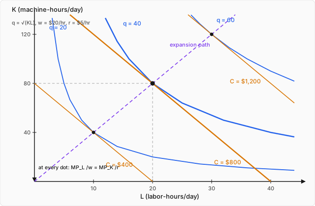
Solve it for the bottling plant. With $w = 20$ and $r = 5$, tangency requires $K/L = w/r = 4$, so $K = 4L$ at every cost-minimizing point regardless of the target output — a fact worth pausing on, since it means the ratio of inputs the firm buys does not depend on how much it is making, only on the price ratio. Substitute into the production function:

At $q = 40$: $L^* = 20$, $K^* = 80$. Check the tangency directly: $MRTS(80,20) = K^*/L^* = 80/20 = 4 = w/r$. ✓ And check the constraint: $\sqrt{80 \times 20} = \sqrt{1600} = 40$. ✓

Conditional factor demands and the cost function, in full

$L^*(w,r,q)$ and $K^*(w,r,q)$ — input demand as a function of prices and the output target, holding cost minimization fixed — are called conditional factor demands, "conditional" because they answer "cheapest way to hit this output" rather than "how much should the firm produce." Do the general Cobb-Douglas case, $q = K^aL^b$, because the specific bottling-plant numbers above are the case $a = b = \tfrac12$, and the general result is what actually explains where $TC(q)$ comes from.

Take logs of the constraint — legitimate because $\ln$ is strictly increasing, so it does not change which bundles satisfy $f(K,L) = q$, only how the equation is written:

(This is the identical trick Consumer Choice used, just applied to the other half of the problem. There, the objective was Cobb-Douglas and the constraint was linear, so logging the objective simplified things. Here the cost objective $wL + rK$ is already linear and the constraint is Cobb-Douglas, so logging the constraint is the move — same trick, mirrored across the problem.) The Lagrangian is

with first-order conditions

Substitute both into the logged constraint:

and solving for $\mu$:

with the conditional factor demands falling out immediately as $K^* = \mu a/r$ and $L^* = \mu b/w$, and total cost as

This is the payoff the whole topic has been aiming at: a cost function derived, not assumed, built entirely out of the production technology and the two input prices. Verify it reduces to the bottling-plant numbers found geometrically above. With $a = b = \tfrac12$, so $a+b=1$:

At $w=20$, $r=5$, $q=40$: $\mu = 2(40)\sqrt{100} = 80 \times 10 = 800$. Then $C = (a+b)\mu = 800$, $K^* = \mu a/r = 800(0.5)/5 = 80$, $L^* = \mu b/w = 800(0.5)/20 = 20$. All three match the direct calculation exactly. ✓ And since $a+b=1$ here, $C(w,r,q) = 2q\sqrt{wr}$ is linear in $q$: cost per unit is the constant $2\sqrt{wr} = 20$ dollars regardless of scale — so $MC(q) = ATC(q) = 20$ for every output. That flat marginal-equals-average cost is not a coincidence of arithmetic; the next section shows exactly which feature of the technology produces it.

One more structural fact is worth isolating before moving on, because it is the input-side twin of a result Consumer Choice found on the demand side. From $K = \mu a/r$ and $L = \mu b/w$: $rK^* = \mu a$ and $wL^* = \mu b$, so

constant expenditure shares on inputs, fixed by the exponents alone and independent of $w$, $r$, and $q$ — exactly the constant-expenditure-share result Cobb-Douglas utility produced for a consumer's spending on goods, now showing up on a firm's spending on inputs. It is the same functional form doing the same thing on both sides of the same market.

Returns to scale and the shape of long-run average cost

The bottling plant's technology, $q = K^{1/2}L^{1/2}$, has $a + b = 1$. Scale both inputs by a factor $\lambda$: $f(\lambda K, \lambda L) = (\lambda K)^a(\lambda L)^b = \lambda^{a+b}f(K,L)$. So $a+b$ is exactly the answer to "if I double every input, what happens to output?" — increasing returns to scale if $a+b>1$ (output more than doubles), constant returns if $a+b=1$ (output exactly doubles), decreasing returns if $a+b<1$ (output less than doubles).

And $a+b$ shows up again, immediately, in the cost function: from the boxed formula, $C(w,r,q) \propto q^{1/(a+b)}$, so long-run average cost is

The exponent's sign is entirely controlled by $a+b$ versus $1$. Constant returns ($a+b=1$) give exponent zero — a flat $LRAC$, exactly what the bottling plant showed above. Increasing returns ($a+b>1$) give a negative exponent — $LRAC$ falls as $q$ grows, without bound. Decreasing returns give a positive exponent and a rising $LRAC$.

That falling case is worth seeing in numbers, because it is the textbook condition for a natural monopoly: if bigger is always cheaper per unit, the single firm that gets there first can underprice any rival forever, and splitting the market between two producers is strictly wasteful. Take a technology with $a=b=\tfrac23$ (so $a+b = \tfrac43$, increasing returns) and, to keep the arithmetic clean, equal input prices $w=r=1$. Tangency gives $K/L = (a/b)(w/r) = 1$, so $K=L$, and the constraint becomes $q = (K\cdot K)^{2/3} = K^{4/3}$, so $K^* = L^* = q^{3/4}$. Choosing $q = n^4$ makes this an exact integer, $K^*=L^*=n^3$, with cost $C = K^*+L^* = 2n^3$ and

Average cost keeps falling as the operation grows, with no floor — precisely because doubling both inputs more than doubles output, so the same proportional increase in spending buys a disproportionately larger increase in output.

Now connect this back to where the whole track's cost apparatus started. Costs of Production found long-run average cost for Amara's bakery by an entirely different route — no isoquants, no Lagrangian, just replicating identical fixed-size ovens and counting — and landed on a perfectly flat $10-per-loaf curve. That flatness was not a coincidence of the bakery's particular numbers; it was constant returns to scale, arrived at by a replication argument instead of the $a+b$ condition derived here. Two completely different techniques — one counting physical ovens, one differentiating a Cobb-Douglas Lagrangian — landing on the identical shape of curve, because they are describing the identical economic fact from two directions.

Shephard's lemma: differentiating cost to get quantity

Here is a genuinely strange-looking claim, worth stating before it is proven so the proof has something to surprise you: differentiate the cost function with respect to an input's price, and what falls out is not a cost at all — it is a quantity, the conditional demand for that very input.

This is Shephard's lemma, and it deserves the envelope-theorem argument rather than a citation. Write cost at the optimum as $C(w,r,q) = wL^*(w,r,q) + rK^*(w,r,q)$, and differentiate the whole right side with respect to $w$, product rule and all — remembering that $L^*$ and $K^*$ are themselves functions of $w$:

The claim is that the last two terms cancel each other exactly. Here is why. The optimal bundle sits on the target isoquant for every value of $w$, so $f\big(K^*(w),L^*(w)\big) = q$ holds identically — differentiate both sides with respect to $w$:

Now bring in the first-order conditions from cost minimization, $MP_K = r/\lambda$ and $MP_L = w/\lambda$ (where $\lambda$ is the multiplier on the original, non-logged constraint $f(K,L)=q$ — it is the shadow price of relaxing that constraint, which is exactly marginal cost, $\lambda = MC(q)$). Substitute:

which is precisely the pair of terms that needed to vanish. What makes them vanish is not an accident of algebra — it is that at a cost-minimizing point, a first-order change in how the firm buys $q$ costs nothing at the margin, because the firm was already choosing that mix optimally. Only the direct effect of $w$ on the wage bill survives, leaving $\partial C/\partial w = L^*$.

Check it on the bottling plant. $C(w,r,q) = 2q\sqrt{wr}$, so

At $w=20$, $r=5$, $q=40$: $\partial C/\partial w = 40\sqrt{5/20} = 40(0.5) = 20$ — and $L^*$ computed directly, earlier, was also $20$. ✓ Differentiating a dollar figure with respect to another dollar figure produced a headcount, and it was the right headcount.

Short run versus long run: the envelope

Every conditional factor demand above assumed both $K$ and $L$ are free to adjust. In the short run, capital is stuck — leased, installed, not renegotiable before next quarter — at whatever level $\bar K$ the firm committed to. Producing $q$ then means finding whatever $L$ makes $f(\bar K, L) = q$, with no freedom to also move $K$, so short-run cost is cost minimization with one fewer degree of freedom:

with equality only at the one output $q_0$ for which $\bar K$ happens to equal the true optimum $K^*(w,r,q_0)$. Off that output, the firm is stuck paying for either too much or too little capital relative to what it would freely choose, so it can only be worse off — it is minimizing over a smaller choice set than the long run allows, and a constrained minimum can never beat an unconstrained one over the same objective.

Suppose the bottling plant commits to $\bar K = 80$ machine-hours a day — the capital level that was exactly optimal for $q=40$. For any other output, solve $\sqrt{80\,L} = q$ for $L = q^2/80$, giving

At $q=40$: $SC(40) = 1600/4 + 400 = 800$, matching the long-run $C(40) = 800$ exactly — equality, as it must be, since $\bar K=80$ is $K^*(40)$. At $q=60$, off that output: $SC(60) = 3600/4 + 400 = 1{,}300$, while the long-run minimum is $C(60) = 20(60) = 1{,}200$. The plant pays 100 dollars a day more than it would if it could also resize its machine fleet — the cost of being stuck at yesterday's capital plan.

The relationship is not just equal levels at $q=40$; it is a genuine tangency. Differentiate: $SC'(q) = q/2$, so $SC'(40) = 20$, and the long-run $MC = 20$ at every output (constant returns, flat curve). Same slope, same level, at exactly $q=40$ — the short-run curve touches the long-run curve there and lies strictly above it everywhere else. Run this same construction for every possible $\bar K$ — one short-run curve per capital commitment, each one minimized at the output for which that particular $\bar K$ happens to be optimal — and the long-run average cost curve is the lower envelope of all of them, not a curve drawn separately and asserted to sit underneath, but the literal boundary traced by the best available short-run plan at every output. When the technology has constant returns, as here, that envelope degenerates to a flat line, and every short-run $U$-shaped curve dips down to kiss it and rises away again — which is exactly the shape Costs of Production drew, from the ovens-and-replication side, when its own long-run curve sat flat at $10 while each individual oven's short-run $ATC$ was a proper $U$.

Worked example

Where this leads

Start from a two-input production function, apply the same Lagrangian that solved a consumer's problem two topics ago, and everything Costs of Production took as given falls out with a derivation behind it: the tangency condition $MP_L/w = MP_K/r$, conditional factor demands built in full on Cobb-Douglas, a cost function $C(w,r,q)$ that explains where $TC(q)$ actually comes from, returns to scale mapping directly onto whether long-run average cost falls, sits flat, or rises, Shephard's lemma turning a cost derivative into a headcount, and a short-run cost curve proven — not drawn and asserted — to sit tangent to the long-run envelope at exactly one output. The bakery's flat $10 curve and the natural-monopoly case of ever-falling average cost are now the same equation, $LRAC \propto q^{1/(a+b)-1}$, evaluated at two different values of $a+b$.

But notice everything this topic held fixed. $w$ and $r$ sat on the page as data throughout — numbers the firm reacts to, never numbers it explains. What happens to a firm's whole cost structure, and therefore to its position in Firms in Competitive Markets, when the wage it faces actually changes — a citywide raise, a new machine-rental market opening up two counties over? Shephard's lemma already contains half the answer, since it says exactly how conditional demand for each input responds to its own price, but nothing here has asked where $w$ and $r$ themselves settle.

That question turns out to be the same one left standing at the end of Consumer Choice. Both halves of every market in this track have now been solved — Nadia optimizing against prices $p_x, p_y$ she cannot move, this bottling plant optimizing against prices $w, r$ it cannot move — and both solutions treated their prices as arriving from outside, on a sign, unexplained. But every one of those prices is itself the outcome of some other market clearing: the labor market that sets $w$ is made of firms like this one demanding labor and people like Nadia supplying it, simultaneously. Solve every market at once, consumers and firms and all, and the prices stop being data and become unknowns to be found — along with two theorems about whether what comes out the other end is any good. That is General Equilibrium and the Welfare Theorems.