Firms in Competitive Markets

Amara's bakery sells bread at $12 a loaf. She did not choose that number and she cannot change it: there are five hundred bakeries in the city selling the same plain white loaf, and $12 is what the loaf goes for. If she asks $12.50 her customers walk two streets over. If she asks $11.50 she sells out by ten in the morning and leaves money on the counter. So the price is simply a fact of her day, like the weather.

What she does choose is how many loaves to bake. And here she had an argument with herself last month, which she settled by trying three different Thursdays.

The previous topic worked out her costs completely. Her total cost of baking $q$ loaves is $TC(q) = 400 + q^2/16$ dollars a day, her cost per loaf is $ATC(q) = 400/q + q/16$, and that cost per loaf bottoms out at $10 when she bakes exactly 80 loaves. Eighty is her efficient scale — the quantity at which a loaf costs her as little as a loaf can possibly cost. So the first Thursday she baked 80. Each loaf cost $10 and sold for $12, a margin of $2 a loaf, and she cleared

The second Thursday she baked 96. Now her cost per loaf was $400/96 + 96/16 = 4.1\overline{6} + 6 = 10.1\overline{6}$ dollars — worse than before, a thinner margin of $1.83 a loaf. And yet:

Sixteen dollars more, from bread that cost more per loaf to make. The third Thursday she pushed to 112 loaves, cost per loaf $400/112 + 7 = 10.57$ dollars, margin $1.43, and cleared

back to exactly where 80 loaves had put her. Not approximately — exactly, to the cent.

Two things here are strange, and they are the whole subject of this topic. First, the quantity that makes bread most cheaply is not the quantity that makes the most money, which sounds almost like a contradiction until you see why. Second, 80 and 112 tie precisely, and 96 sits precisely between them. That is not an accident of the numbers Amara happened to try; it is a fingerprint of the shape of the profit function, and once you see the shape you can read off the answer without trying any Thursdays at all.

What a price taker actually faces

Before differentiating anything, be precise about the situation, because the whole derivation turns on one assumption.

Amara is in a perfectly competitive market. Three conditions define it: there are many buyers and many sellers, the good they trade is identical from seller to seller, and firms are free to enter or leave the industry. The first two conditions together mean no single seller's decisions move the price. The third one matters later, and it is what drives the long run.

"No single seller moves the price" deserves better than an assertion, because it is not exactly true — it is approximately true, and it is worth knowing how approximately. Suppose the city's demand for bread is

loaves a day. At $12 that is 48,000 loaves, which is 500 bakeries selling 96 each — Amara's Thursday, and the whole city's. Now suppose Amara doubled her output to 192 loaves. The market quantity would rise by 96 loaves, and to clear that extra bread the price would have to fall by

about three cents. She does move the price. She moves it by a quarter of one percent, which is less than the day-to-day noise in her flour bill. Treating $P$ as a constant she cannot affect is not a fairy tale about her having no power; it is a statement that her power is small enough to round to zero, and we can say exactly how small.

With $P$ constant, the firm's revenue is trivially simple:

Two derived quantities follow, and they collapse into each other in a way that is special to competition. Average revenue is revenue per unit, $AR = R/q = P$. Marginal revenue is the extra revenue from one more unit,

For a price taker, $P = AR = MR$. Hold on to how this happens, because it is the exact place where a monopoly will differ. In general a firm's revenue is $R = P(Q)\,q$, where the price depends on how much is sold, and the product rule gives

Selling one more loaf brings in $P$ dollars from that loaf, and costs you $q \times dP/dq$ dollars because the extra supply nudges the price down on every loaf you were already selling. For Amara the second term is $96 \times (-1/3{,}000) = -0.032$ dollars: it exists, and it is nothing. Set it to zero and $MR = P$.

The picture of the firm's own demand curve is worth carrying: while the market demand curve slopes down, the demand curve facing a single price-taking firm is a horizontal line at the market price. She can sell 10 loaves or 200 at $12; she can sell none at all at $12.01.

Produce until marginal cost equals the price

Now the derivation. Profit is revenue minus total cost,

and Amara wants the $q$ that makes this as large as possible. Differentiate and set to zero:

That is the general rule for any firm whatsoever, competitive or not: produce until the last unit's revenue exactly equals the last unit's cost. For a price taker, $MR = P$, and it specializes to

The economics underneath the calculus is a one-sentence argument, and it is worth being able to make without the derivative. If $P > MC$, the next loaf brings in more than it costs, so baking it adds to profit — bake it. If $P < MC$, the last loaf cost more than it brought in, so not baking it adds to profit — don't. The only place you can stop and not want to move is where they are equal.

Apply it to the bakery. Her marginal cost, derived last topic, is $MC(q) = q/8$, so

There is Amara's second Thursday, produced from the rule rather than from experiment. And now the first strangeness dissolves. At $q = 80$, her efficient scale, marginal cost is $MC(80) = 80/8 = 10$ dollars. The eighty-first loaf costs her ten dollars and something to bake, and sells for twelve. Of course she should bake it. Efficient scale is the answer to the question "at what output is bread cheapest per loaf?" — a question about the cost curves alone, in which the price never appears. Nothing obliges the answer to a cost question to also be the answer to a profit question. Baking past 80 raises her average cost, and she does it anyway, because each extra loaf is still individually worth baking.

The second strangeness — the exact tie between 80 and 112 — falls out of completing the square. Write the profit function out:

A downward parabola with its vertex at $q = 96$ and a maximum of $176 a day. Every quantity is penalized by $(q-96)^2/16$, which depends only on the distance from 96. Since $80$ and $112$ are both 16 loaves away, both lose $16^2/16 = 16$ dollars, landing both on $176 − $16 = $160. The tie was inevitable. (Check that this parabola really is her profit: expanding gives $176 - (q^2 - 192q + 9216)/16 = 176 - q^2/16 + 12q - 576 = 12q - q^2/16 - 400$. ✓)

The general version is just as clean. With $TC(q) = F + q^2/16$ and any price $P$,

The vertex sits at $q = 8P$, which is the $P = MC$ rule again, and the maximum profit is

At $P = 12$ and $F = 400$ that is $4(144) - 400 = 176$ dollars. ✓ Keep this formula; it will do a lot of work in a moment.

The second-order condition, and why half the marginal cost curve is a trap

Setting a derivative to zero finds stationary points, not maxima. Finish the job:

Profit is concave — the stationary point is a genuine maximum — if and only if marginal cost is rising there. Where marginal cost falls, $\pi'' > 0$ and the point where $P = MC$ is a local minimum of profit: the worst output in its neighborhood, not the best.

For Amara this is invisible, because her marginal cost $q/8$ rises from the first loaf. But recall the pottery studio from the previous topic's worked example, whose costs were

That marginal cost curve is U-shaped: $MC'(q) = -1 + 0.3q$, so $MC$ falls until $q = 10/3$ and rises after. Put the studio in a market where bowls sell for $9.40 and look for the outputs satisfying $P = MC$:

Two solutions, both exact. The rule "produce where $P = MC$" does not, by itself, tell you which. So compute the profit at each, and at the third option of baking nothing at all. Variable cost at $q = 6$ is $60 - 18 + 10.8 = 52.8$:

At $q = \tfrac{2}{3}$, variable cost is $6.\overline{6} - 0.\overline{2} + 0.0148 = 6.4593$:

And at $q = 0$ the studio earns nothing and still pays its $50 fixed cost, so $\pi(0) = -50$ dollars.

Rank them: $-46.40 > -50 > -50.19$. The output on the rising branch of $MC$ is the best of the three. The output on the falling branch is the worst — worse even than shutting the kiln down entirely. Exactly as the second-order condition promised: $MC'(2/3) = -1 + 0.2 = -0.8$, so $\pi''(2/3) = +0.8 > 0$, a local minimum; while $MC'(6) = -1 + 1.8 = 0.8$, so $\pi''(6) = -0.8 < 0$, a local maximum.

This is why the textbook sentence is always "the supply curve is the upward-sloping portion of marginal cost". It is not a drafting convention or a simplification. The downward-sloping portion solves the same equation and gives the answer that loses the most money.

When to stop: the shutdown rule

The pottery calculation just did something the $P = MC$ rule cannot do on its own: it compared the best interior output against the option of producing nothing. That comparison is a separate decision with its own rule, and the rule is not the one most people guess.

The naive guess is "shut down if you are losing money". At $9.40 a bowl the studio loses $46.40 a day and should nevertheless keep the kiln lit. Here is the derivation of the actual rule.

Write total cost as fixed plus variable, $TC(q) = FC + VC(q)$. Producing $q$ units yields

Shutting down means $q = 0$: no revenue, no variable cost, and — in the short run — the fixed cost regardless, because the lease is signed and the insurance is paid whether the door opens or not. So

Produce if $\pi_{\text{produce}} \ge \pi_{\text{shut}}$:

The fixed cost cancels. It appears identically on both sides of the comparison, which is the formal statement of the fact established last topic — fixed cost is invisible at the margin, and here it turns out to be invisible in the shutdown decision too. A cost you pay either way cannot be a reason to choose either way. Economists call such a cost sunk, and the whole content of the shutdown rule is: ignore sunk costs.

What the firm compares instead is price against average variable cost: does each unit at least pay for the ingredients and labor that went into it? If it does, the surplus $P - AVC$ per unit is a contribution toward the fixed cost you are stuck with anyway. Check the studio: $AVC(6) = 10 - 3 + 1.8 = 8.80$ dollars, and

which turns a $50 loss into a $46.40 loss. ✓ Exactly the $3.60 gap computed above. The studio is not making money; it is losing less money, and that is the correct thing to do.

Since $MC$ cuts $AVC$ at the bottom of $AVC$ — the theorem proved in the previous topic — the firm operating on the rising branch of $MC$ has $P = MC \ge AVC$ exactly when $P$ is at least the minimum of average variable cost. So the rule can be stated once, in terms of the curves rather than the chosen quantity:

For the pottery studio, $AVC' = -0.5 + 0.1q = 0$ gives $q = 5$ and $AVC(5) = 10 - 2.5 + 1.25 = 8.75$ dollars. At $9.40 the studio is above that and should produce, as we found. Drop the price to $8.60 and it falls below: the arithmetic then gives an optimal interior output of $q = 14/3$, where $AVC(14/3) = 10 - 2.\overline{3} + 1.0\overline{8} = 8.756$ dollars — above the price — so each bowl loses 15.6 cents on its own variable cost, and $\pi = -50.73$ dollars is worse than the $50 loss of shutting. ✓ The rule and the direct comparison agree.

The long run is different in exactly one respect, and it is the respect that matters. Over a long enough horizon nothing is sunk: the lease expires, the oven can be sold, the license lapses. A firm choosing whether to be in the industry at all avoids every cost by leaving, so the comparison becomes $Pq - TC(q) \ge 0$, which by the same one-line division is

Two rules, one derivation, one difference: which costs are still avoidable. That is the entire content of "the short run is when some inputs are fixed". A firm can therefore sit for years in the band $AVC_{\min} \le P < ATC_{\min}$ — losing money every single day, correctly refusing to close today, and correctly planning to be gone when the lease runs out.

The supply curve, at last

Everything needed for a supply curve is now proved. A price-taking firm's chosen output at price $P$ is the solution of $P = MC(q)$ on the rising branch, provided $P \ge AVC_{\min}$; otherwise it is zero. Read that sentence sideways and it is a supply curve — a rule assigning a quantity to each price:

The firm's supply curve is its marginal cost curve above minimum average variable cost. Not something derived from it, not something resembling it — the same curve, with the axes read in the other order.

For Amara, $MC(q) = q/8$, so

Her average variable cost is $AVC = q/16$, which slides down to zero as $q$ does, so her shutdown price is zero: there is no positive price at which she prefers a dark bakery. That is a peculiarity of a cost function with no fixed labor requirement, and the pottery studio above shows the general case, where the shutdown price is a real and positive $8.75.

The market supply curve is the horizontal sum of the firms' supply curves: at each price, add up the quantities, not the prices. (Horizontal, because price is the thing they have in common and quantity is the thing being pooled. This is the mirror image of the vertical summation used for public goods, where the quantity is what everyone shares and the willingness to pay is what gets added.) With 500 bakeries identical to Amara's,

Which is the number the previous topic asserted and left hanging. It is now earned: it slopes upward because marginal cost rises, marginal cost rises because the marginal product of labor falls, and the marginal product of labor falls because there is only one oven. The upward-sloping supply curve that Supply, Demand, and Market Equilibrium drew on faith has been traced all the way back to a crowded kitchen.

When firms are not identical, the sum acquires kinks. A firm with a shutdown price of $8 contributes nothing below $8 and joins the sum above it, so the market supply curve bends outward each time a new group of firms switches on. Nothing about the derivation changes; the curve just stops being smooth.

And now check the market clears at the price we assumed all along. Setting $Q^S = Q^D$:

with $Q = 48{,}000$ loaves, or 96 per bakery. ✓ Amara's $12 was not handed down; it is what 500 bakeries with these costs and this demand produce between them.

Amara's $324, and what the industry does about it

Everything so far used Amara's explicit costs — the money that leaves her account. The previous topic insisted, at some length, that this is the wrong cost function to make decisions with. She owns her storefront outright, forgoing $150 a day in rent she could collect from a tenant, and she works in the bakery instead of consulting for $350 a day. Those $500 a day of implicit costs are as real as flour. They are also fixed — she gives them up whether she bakes 10 loaves or 200 — so the economically correct cost function is

with the same marginal cost $MC = q/8$ (adding a constant changes nothing at the margin, which is why her output choice of 96 loaves stands unchanged) but a different average total cost, $ATC(q) = 900/q + q/16$.

Now use the formula derived above, $\pi^{\max}(P) = 4P^2 - F$, twice:

Both numbers exactly as the previous topic reported them, now falling out of one line of algebra. And they can be read off a diagram, because economic profit has a geometric shape. Since $\pi = Pq - TC(q)$ and $TC = ATC \times q$,

a rectangle: height the gap between price and average total cost, width the quantity. At $q = 96$, $ATC(96) = 900/96 + 6 = 15.375$ dollars, so the height is $12 - 15.375 = -3.375$ dollars — a negative height, which is to say the rectangle sits above the price line — and

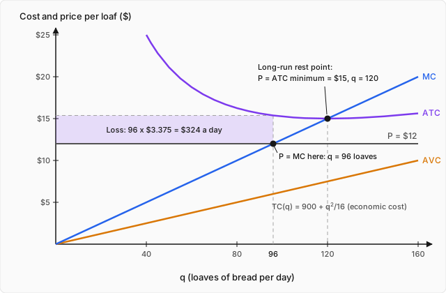
Look at what the diagram says that a table of numbers does not. The purple $ATC$ curve never touches the price line — its lowest point is at $15, and the price is $12. There is no quantity whatsoever at which Amara covers her economic costs. She is not producing the wrong amount; 96 is genuinely her best available choice. The problem is that her best available choice is a loss.

And she is not special. All 500 bakeries have the same costs, so all 500 are losing $324 a day, which is $162,000 a day of value being destroyed across the industry. That is a great deal of pressure, and here is where the third defining condition of competition — free entry and exit — finally does its work.

Entry, exit, and the long-run resting point

Some bakers give up. Their leases lapse and they do not renew, they sell their ovens, they go back to consulting. Suppose 175 of the 500 leave. Market supply is now the horizontal sum of 325 firms:

and the new equilibrium is

The mechanism is worth stating in words, because it is easy to lose in the algebra: fewer sellers means less bread at any given price, which means the supply curve shifts left, which means it meets the unchanged demand curve at a higher price. The exit of some firms raises the price for the survivors. Nobody intended this and nobody coordinated it; each departing baker was just cutting her own losses.

Now check what $15 does to a survivor. She produces $q = 8(15) = 120$ loaves, and her profit is

Zero. Exactly zero, and the process stops there — no one else has any reason to leave. The system has found a rest point.

It rests from the other side too. Suppose instead the industry had only 150 bakeries. Then $Q^S = 1{,}200P$, and $1{,}200P = 84{,}000 - 3{,}000P$ gives $P = 20$ dollars, at which each bakery produces 160 loaves and earns $4(400) - 900 = 700$ dollars a day of economic profit — $700 a day better than the best alternative use of those resources. That is a signal visible to anyone with a spreadsheet, and new bakeries open. Every entrant shifts supply right and pushes the price down, and entry continues until the profit is gone, which is to say until $P = 15$ dollars again.

Free entry and exit drive economic profit to zero. Now watch what that does to the individual firm, because it is a much stronger statement than it looks. Zero profit means

With $F = 900$, $P = 15$ dollars. But the previous topic computed the bakery's minimum average total cost in general and got

The same expression. The long-run price is not merely near the bottom of the average cost curve; it is equal to it, identically, for every $F$. And then the quantity each firm chooses is

its efficient scale. With $F = 900$: $P = 15$ dollars and $q = 120$ loaves, which is the second dot on the diagram — the point where $MC$ passes through the minimum of $ATC$.

This is the payoff of the theorem proved last topic, and it deserves to be spelled out. Marginal cost cuts average total cost exactly at the bottom of $ATC$, so the single point $P = MC = ATC_{\min}$ satisfies both conditions at once: the firm is maximizing profit ($P = MC$) and earning exactly zero ($P = ATC$). No other price can satisfy both. So competition, which nobody designed and no one administers, ends by pushing every surviving bakery to the exact quantity at which bread is made as cheaply as it can be made. Amara's opening puzzle — that 80 is the cheapest quantity but 96 the most profitable — was a symptom of a market out of equilibrium. Once the price has settled, the cheapest quantity and the most profitable quantity are the same quantity.

Finally, the head count. Demand at $15 is $84{,}000 - 45{,}000 = 39{,}000$ loaves, and each bakery makes 120, so

The 175 that left were not driven out by anyone's bad baking. They were the arithmetic surplus of an industry that had more capacity than the city's appetite for bread would pay for.

Why the long-run supply curve is flat

Push on the resting point once more. The long-run price is $\sqrt{F}/2 = 15$ dollars, and notice what does not appear in that expression: demand. Not the intercept, not the slope, nothing. The long-run price is determined entirely by the firms' cost function.

So ask what happens if the city's appetite for bread grows — a new neighborhood, say — shifting demand to

In the short run the 325 existing bakeries cannot multiply, and their supply is still $Q^S = 2{,}600P$:

Each bakery slides up its own marginal cost curve to $q = 8(18) = 144$ loaves and earns $4(324) - 900 = 396$ dollars a day. But that profit is precisely the signal that summons entrants, and entry proceeds until the price is back to $15. At $15, demand is $100{,}800 - 45{,}000 = 55{,}800$ loaves, and at 120 loaves each that needs

A hundred and forty new bakeries, and the price ends exactly where it started. Plot the long-run relationship between market quantity and price and you get a horizontal line at $15: the long-run market supply curve is flat. Quantity adjusts through the number of firms, not through the price. An industry that behaves this way is called a constant-cost industry.

There is a satisfying consistency check available here. The previous topic worked out Amara's long-run cost directly, by letting her lease $n$ ovens and replicating the best small plant; with a fixed cost $F$ per plant, that gave a flat long-run average cost equal to $\sqrt{F}/2$ per loaf. The market's long-run supply price and the firm's long-run average cost are the same number for the same reason — free entry replicates efficient plants until the market is served, exactly as the single firm replicated ovens until its own output was served.

Two honest caveats. First, the flatness depends on new entrants having the same costs as incumbents. If expansion bids up the price of an input — skilled bakers become scarce, commercial ovens back-order, storefront rents rise — then every firm's cost curves shift up as the industry grows, $ATC_{\min}$ rises with output, and the long-run supply curve slopes gently upward. That is an increasing-cost industry, and it is the common case; the argument is unchanged apart from $F$ becoming a function of industry size. Second, "long run" here means whatever horizon lets leases lapse and new ovens arrive. Nothing in the derivation says it is quick.

Zero profit is not zero profit

One thing about the resting point still sounds wrong, and it is worth killing properly. If competition drives economic profit to zero, why does anyone stay in business?

Because zero economic profit is not zero accounting profit — the distinction the previous topic built and this one has been quietly living off. Run Amara's books at the long-run equilibrium, $P = 15$ dollars and $q = 120$ loaves:

Her accountant reports a profit of $1{,}800 - 1{,}300 = 500$ dollars a day — about $180,000 a year. Her economist reports

because the $500 of implicit costs — the rent she is not collecting and the consulting salary she is not earning — is exactly what her accounting profit comes to. That is not a coincidence; it is what zero economic profit means. She is earning precisely what her building and her working day are worth in their best alternative use, no more and no less.

So the long-run equilibrium is not a place where firms are wretched. It is a place where nothing is being wasted: no resource is stuck in an industry that values it less than somewhere else does, and none is being drawn away from an industry that values it more. And it explains a fact about real competitive industries that otherwise looks like a paradox — that people run bakeries and hardware stores and haulage firms for decades, making a perfectly respectable living, without ever getting rich. The respectable living is the implicit cost. The not getting rich is the zero economic profit.

Worked example

Where this leads

Start with the assumption that a firm cannot move the price, and everything else in this topic is forced. Profit maximization gives $P = MC$; the second-order condition throws away the falling branch of $MC$ and keeps the rising one; the surviving branch, read sideways, is the firm's supply curve; horizontal summation makes it the market's; and free entry and exit push the price down to the bottom of the average cost bowl, where every firm produces at efficient scale and earns exactly what its resources would have earned elsewhere. The supply curve that was drawn on faith five topics ago, and whose costs were opened up in the costs of production, is now derived from a production function and a wage.

That is a genuinely remarkable result, and it is worth naming what makes it remarkable: nobody in the story is trying to achieve it. Amara is not trying to bake bread cheaply for the city; she is trying to have a good day. The 175 bakers who left were not making room for anyone; they were cutting their losses. The outcome — every loaf produced at the lowest cost anyone knows how to achieve, sold at that cost — is a by-product. It is the sharpest version yet of what consumer and producer surplus showed about the efficiency of competitive markets, and it is the strongest case that will ever be made for leaving a market alone.

Which is exactly why the assumption at the top deserves suspicion. Every line above used $MR = P$, and $MR = P$ came from dropping the term $q\,dP/dq$ in

We dropped it because Amara's 96 loaves were a rounding error in a 48,000-loaf market — the term was worth three cents. But suppose a single firm is the market. Then $q = Q$, the neglected term is not a rounding error but a substantial subtraction, and marginal revenue falls strictly below price at every output. The rule $MR = MC$ survives, because it was never about competition; the rule $P = MC$ does not. And once price exceeds marginal cost, there are buyers willing to pay more than the cost of serving them who go unserved — the same triangle of destroyed value that turned up in the deadweight loss of a tax and again in externalities, arriving this time from a third direction entirely.

So: what does a firm do when it can choose its price? That is monopoly, and it is where this goes next.