The Costs of Taxation: Deadweight Loss

Imagine the town council of a small farming town — call it Harbor Falls — debating a new tax: five dollars on every bushel of wheat sold in the county, collected from the sellers. The treasurer's arithmetic sounds airtight. The county trades about fifty thousand bushels a year; at five dollars a bushel, the tax simply moves a couple of hundred thousand dollars from the pockets of farmers and millers into the town treasury, where it will be spent on roads and schools. Money out of one pocket, money into another. Nothing created, sure — but surely nothing destroyed either?

A farmer at the hearing raises her hand and objects, but not for the reason you'd expect. She doesn't complain about paying. She points out that at the higher price the tax will force, the miller she sells her last truckload to every autumn won't buy it at all — and that truckload of wheat, which used to become bread, will simply never be grown, milled, or eaten. The town won't collect five dollars on it either, because a sale that doesn't happen yields no tax. That truckload's worth of value — the miller's enjoyment of it and her profit from growing it — won't be transferred to anyone. It will just not exist.

That is the puzzle this topic answers rigorously. A tax looks, at first glance, like a pure transfer — and most of it is. But wrapped inside every tax is a second, quieter effect: it changes the number of trades that happen at all, and the trades it prevents are not moved from one person to another. They are erased. Economists call the value that disappears this way the deadweight loss of the tax — "deadweight" because it benefits no one, not even the government that levied the tax.

The tools to measure it precisely are already in hand. From the consumer and producer surplus topic, we know how to put a dollar figure on the benefit buyers and sellers each get from a market: the areas under the demand curve and above the supply curve, up to the quantity traded. From the price-controls-and-taxes topic, we know exactly what a per-unit tax does to our wheat market — demand $Q_d = 100 - 4P$ , supply $Q_s = -20 + 6P$ (quantities in thousands of bushels) — whose free equilibrium sits at $P^* = 12$ , $Q^* = 52$ , and which, under a $t = 5$ tax on sellers, splits into a buyer price of $15$ , a seller net price of $10$ , and only $40$ thousand bushels traded. The question is: how much of the old total surplus survives, how much becomes tax revenue, and how much is simply gone? And once we can compute that, two deeper questions follow: how fast does the loss grow as the tax grows, and what property of a market makes the loss big or small?

What a "wedge" does to a market

Before any algebra, get the mechanism completely clear in plain words, because the whole topic is one idea: a tax drives a wedge between what buyers pay and what sellers receive, and the wedge decides how much gets traded.

Without a tax, the buyer's price and the seller's price are the same number — the single market price — and trade expands until the very last bushel whose value to some buyer still covers its cost to some seller has been sold. With a tax of $t$ per bushel, the two prices split apart: the buyer pays $P_b$ , the seller keeps only $P_s = P_b - t$ , and the government pockets the $t$ difference on every unit sold. Now the quantity traded has to satisfy two masters at once: it must be the amount buyers are willing to buy at the full price $P_b$ , and simultaneously the amount sellers are willing to sell at the reduced price $P_s$ . Both conditions can hold only at a smaller quantity than before, because pushing the buyer price up shrinks demand while pushing the seller price down shrinks supply, and the two meet somewhere below the old equilibrium.

Here is the part that matters most, and it is easy to get wrong. The deadweight loss has nothing to do with the trades that still happen. On those forty thousand bushels, buyers still buy, sellers still sell, the government collects its five dollars — surplus is reshuffled among the three parties, but every dollar of it still exists somewhere. The loss lives entirely in the trades that stopped: the bushels numbered forty-through-fifty-two-thousand, so to speak. Each of those bushels was worth more to some buyer than it cost some seller to produce — that is exactly why they used to trade — yet after the tax they trade no longer, because the wedge now sitting between the two prices is wider than the small margin of benefit those bushels offered. Their would-be surplus is not transferred to the government. It is not transferred to anyone. It vanishes, and the size of what vanishes is precisely the deadweight loss.

Counting the after-tax market honestly

First, recall where the tax equilibrium itself comes from — one line of algebra, since the derivation lives in the price-controls topic. With a $t = 5$ tax levied on sellers, sellers respond to their net price $P_s = P_b - 5$ , so the market clears where quantity demanded at the buyer price equals quantity supplied at the seller net price:

100 - 4P_b = -20 + 6(P_b - 5) \quad\Longrightarrow\quad 150 = 10\,P_b \quad\Longrightarrow\quad P_b = 15,

giving $P_s = 15 - 5 = 10$ and $Q_t = 100 - 4(15) = 40$ (check the supply side: $-20 + 6(10) = 40$ , same number, as it must be). Concretely: buyers now pay fifteen dollars, sellers keep only ten of them, and because each side is responding to a worse price than before, only forty thousand bushels change hands instead of fifty-two.

Now count every dollar of surplus, before and after. The inverse curves are what turn quantities into areas: demand reads $P = 25 - \tfrac14 Q$ (the buyer of the very last bushel values it at exactly $25 - Q/4$ dollars), and supply reads $P = \tfrac{10}{3} + \tfrac16 Q$ (the seller of the last bushel needs at least $\tfrac{10}{3} + Q/6$ dollars to bother). Each surplus is a triangle: consumer surplus is the area under demand and above the price paid, producer surplus is the area below the price received and above supply.

Before the tax (price $12$ , quantity $52$ ):

CS_{\text{old}} = \tfrac12 \times 52 \times (25 - 12) = 338, \qquad PS_{\text{old}} = \tfrac12 \times 52 \times \left(12 - \tfrac{10}{3}\right) = \tfrac{676}{3} \approx 225.33.

TS_{\text{old}} = 338 + \tfrac{676}{3} = \tfrac{1690}{3} \approx 563.33.

Before the tax, the wheat market generates about $563$ thousand dollars of total benefit per period, split between buyers ( $338$ ) and sellers ( $225$ ), with no one else in the picture.

After the tax (buyer price $15$ , seller price $10$ , quantity $40$ ), the same triangle recipe, now applied to the smaller quantity and the two split prices:

CS_{\text{new}} = \tfrac12 \times 40 \times (25 - 15) = 200, \qquad PS_{\text{new}} = \tfrac12 \times 40 \times \left(10 - \tfrac{10}{3}\right) = \tfrac{400}{3} \approx 133.33.

One new entry appears in the ledger: the government. It collects $t = 5$ dollars on each of the $Q_t = 40$ thousand bushels actually sold — and only on those, since unsold bushels yield nothing:

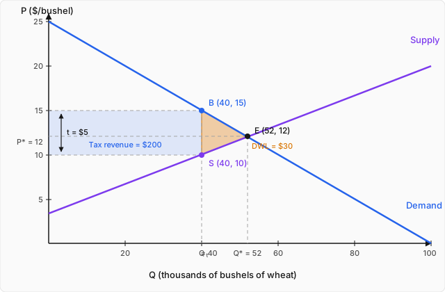
\text{Tax Revenue} = t \times Q_t = 5 \times 40 = 200.

On the graph, the revenue is the rectangle sitting between the seller price and the buyer price, stretching from zero out to the new quantity — height $5$ , width $40$ , area $200$ . Adding up everything that still exists:

TS_{\text{new}} = CS_{\text{new}} + PS_{\text{new}} + \text{Revenue} = 200 + \tfrac{400}{3} + 200 = \tfrac{1600}{3} \approx 533.33.

And now the subtraction that the town treasurer missed:

DWL = TS_{\text{old}} - TS_{\text{new}} = \tfrac{1690}{3} - \tfrac{1600}{3} = \tfrac{90}{3} = 30.

Thirty thousand dollars of value per period — gone, not transferred. The reconciliation is worth doing once explicitly, because it shows exactly where every dollar went. Buyers lost $CS_{\text{old}} - CS_{\text{new}} = 338 - 200 = 138$ ; sellers lost $PS_{\text{old}} - PS_{\text{new}} = \tfrac{676}{3} - \tfrac{400}{3} = \tfrac{276}{3} = 92$ ; together they lost $138 + 92 = 230$ . Of that, $200$ arrived safely in the treasury as revenue. The remaining $230 - 200 = 30$ arrived nowhere. That is the farmer's truckload, scaled up to the whole market.

The deadweight-loss triangle, and a required cross-check

There is a second, cleaner way to compute the same number, and deriving it tells you where the loss sits on the graph. The surplus destroyed is exactly the gap between what those missing bushels were worth to buyers and what they would have cost sellers — bushel by bushel, from $Q_t = 40$ out to $Q^* = 52$ . That is an integral of demand-minus-supply over the missing range:

DWL = \int_{40}^{52} \left[ \left(25 - \tfrac{Q}{4}\right) - \left(\tfrac{10}{3} + \tfrac{Q}{6}\right) \right] dQ = \int_{40}^{52} \left( \tfrac{65}{3} - \tfrac{5Q}{12} \right) dQ.

= \left[ \tfrac{65Q}{3} - \tfrac{5Q^2}{24} \right]_{40}^{52} = \left( \tfrac{3380}{3} - \tfrac{1690}{3} \right) - \left( \tfrac{2600}{3} - \tfrac{1000}{3} \right) = \tfrac{1690}{3} - \tfrac{1600}{3} = 30.

In plain words: integrate the per-bushel benefit that outruns the per-bushel cost over exactly the bushels that stopped trading, and you get back precisely the $30$ from the direct subtraction — the bracket even evaluates to the old and new total surpluses themselves, which is the honest proof that the two methods are the same computation wearing different clothes.

Because the integrand is a straight line falling from $t = 5$ at $Q_t$ (the wedge at the margin is exactly the tax) to $0$ at $Q^*$ (where the curves meet), the integral is just the area of a triangle: height $t$ , base $Q^* - Q_t$ . This gives the formula worth memorizing:

DWL = \tfrac12 \times t \times (Q^* - Q_t) = \tfrac12 \times 5 \times (52 - 40) = \tfrac12 \times 5 \times 12 = 30.

Same $30$ , third time. Put plainly: the deadweight loss is a triangle sitting between the demand and supply curves, wedged between the new quantity and the old one — half the tax times the number of trades killed. Every number in the figure below is one we just computed.

The wheat market under a $5 per-bushel tax: the wedge splits the buyer price ($15) from the seller price ($10), quantity falls from 52 to 40, the government collects the blue rectangle ($200), and the orange triangle between the curves from 40 to 52 — the surplus of the trades that no longer happen — is the deadweight loss, $30.

Why doubling the tax quadruples the damage

So far everything used $t = 5$ specifically. The genuinely important policy result — the one that makes economists nervous about large taxes — only appears when you redo the calculation with a symbol $t$ instead of a number. Take any linear market: inverse demand $P = a - bQ$ , inverse supply $P = c + dQ$ , with $b, d > 0$ . The free equilibrium is where the curves meet:

a - bQ^* = c + dQ^* \quad\Longrightarrow\quad Q^* = \frac{a - c}{b + d}.

With a tax $t$ , the new quantity $Q_t$ is where the gap between the curves exactly equals the tax — buyer price minus seller price must be $t$ :

\left(a - bQ_t\right) - \left(c + dQ_t\right) = t \quad\Longrightarrow\quad Q_t = \frac{a - c - t}{b + d} = Q^* - \frac{t}{b + d}.

What that says: the number of trades killed, $\Delta Q = Q^* - Q_t = \tfrac{t}{b+d}$ , grows proportionally with the tax. Now feed that into the triangle formula:

DWL = \tfrac12 \times t \times \Delta Q = \tfrac12 \times t \times \frac{t}{b+d} = \frac{t^2}{2(b+d)}.

There it is, and it deserves a second look: the tax appears squared. In plain words, the loss grows with the square of the tax because raising the tax does two multiplying things at once — it widens the wedge (the triangle's height, $t$ ) and it kills more trades (the triangle's base, $\tfrac{t}{b+d}$ ) — and area is height times base. Equivalently, the marginal loss from one more dollar of tax, $\dfrac{d\,DWL}{dt} = \dfrac{t}{b+d}$ , is not constant: it grows linearly with the tax already in place. A small tax is nearly free; each additional dollar of tax is more expensive than the last.

Check the formula against the case we already know: with $b = \tfrac14$ , $d = \tfrac16$ , we get $2(b+d) = \tfrac56$ , so $DWL = t^2 / \tfrac56 = \tfrac65 t^2$ , and at $t = 5$ : $\tfrac65 \times 25 = 30$ . Matches. Now make it concrete with a doubled tax, $t = 10$ , on the same wheat market. The clearing condition $100 - 4P_b = -20 + 6(P_b - 10)$ gives $180 = 10P_b$ , so $P_b = 18$ , $P_s = 8$ , and $Q_t = 100 - 72 = 28$ . The triangle:

DWL_{t=10} = \tfrac12 \times 10 \times (52 - 28) = \tfrac12 \times 10 \times 24 = 120,

and the formula agrees: $\tfrac65 \times 100 = 120$ . Doubling the tax from $5$ to $10$ did not double the damage — it quadrupled it, from $30$ to $120$ . This is the single most important quantitative fact about deadweight loss, and it is the rigorous version of a common-sense worry: the cost of a tax system grows much faster than the tax rates themselves.

Deadweight loss and elasticity: which markets suffer most

One question remains: the formula $DWL = \tfrac{t^2}{2(b+d)}$ depends on the slopes $b$ and $d$ — what economic property of a market do those slopes measure? The elasticity topic already built the answer. Elasticity is, at bottom, the derivative of quantity with respect to price, scaled into units-free form: since inverse demand is $P = a - bQ$ , the demand slope in quantity-space is $\dfrac{dQ_d}{dP} = -\dfrac1b$ , and likewise $\dfrac{dQ_s}{dP} = \dfrac1d$ . At the free equilibrium, the price elasticities are therefore

\eta_d = \left|\frac{dQ_d}{dP}\right| \cdot \frac{P^*}{Q^*} = \frac{P^*}{b\,Q^*}, \qquad \eta_s = \frac{dQ_s}{dP} \cdot \frac{P^*}{Q^*} = \frac{P^*}{d\,Q^*}.

Solving each for its slope — $\dfrac1b = \dfrac{\eta_d Q^*}{P^*}$ and $\dfrac1d = \dfrac{\eta_s Q^*}{P^*}$ — and substituting into the quantity response $\Delta Q = \dfrac{t}{b+d}$ :

b + d = \frac{P^*}{Q^*}\left(\frac{1}{\eta_d} + \frac{1}{\eta_s}\right) \quad\Longrightarrow\quad \Delta Q = \frac{t\,Q^*}{P^*\left(\frac{1}{\eta_d} + \frac{1}{\eta_s}\right)}, \qquad DWL = \frac{t^2\, Q^*}{2\,P^*\left(\frac{1}{\eta_d} + \frac{1}{\eta_s}\right)}.

Read it this way: the elasticities sit in the denominator of the denominator — bigger $\eta_d$ or $\eta_s$ makes the parenthesized sum smaller, and so makes the deadweight loss bigger. Verify on the wheat market: $\eta_d = \dfrac{12}{\tfrac14 \times 52} = \dfrac{12}{13}$ and $\eta_s = \dfrac{12}{\tfrac16 \times 52} = \dfrac{18}{13}$ , so $\dfrac{1}{\eta_d} + \dfrac{1}{\eta_s} = \dfrac{13}{12} + \dfrac{13}{18} = \dfrac{65}{36}$ , and

DWL = \frac{25 \times 52}{2 \times 12 \times \frac{65}{36}} = \frac{1300 \times 36}{1560} = 30.

Same $30$ , fourth time — the elasticity formula is the triangle formula, just re-parametrized. The economic meaning is the deep part: elasticity is the responsiveness of quantity to price, and deadweight loss is, literally, the value of the quantity that stops moving. A market where buyers or sellers respond strongly to price — think luxury goods with many substitutes, or labor that can easily be withheld — is a market where a given tax kills many trades, and therefore destroys much value per dollar raised. A market of necessities, where quantity barely budges, yields revenue with little deadweight loss. This is why economists wince at taxes on elastic goods and why, if taxes must exist, they prefer them on inelastic ones.

Worked example

A city's market for concert tickets has demand $Q_d = 200 - 5P$ and supply $Q_s = -40 + 5P$ (quantities in hundreds of tickets, prices in dollars). The city imposes a tax of $t = 8$ dollars per ticket on sellers. Compute the deadweight loss of the tax — by the direct surplus subtraction, and by the triangle formula — and confirm the two agree.

Step 1 — free equilibrium. Set $Q_d = Q_s$ : $200 - 5P = -40 + 5P \Rightarrow 240 = 10P \Rightarrow P^* = 24$ , and $Q^* = 200 - 5(24) = 80$ . Inverse curves: demand $P = 40 - \tfrac15 Q$ , supply $P = 8 + \tfrac15 Q$ .

Step 2 — after-tax equilibrium. Sellers receive $P_s = P_b - 8$ , so the market clears where

200 - 5P_b = -40 + 5(P_b - 8) \quad\Longrightarrow\quad 280 = 10P_b \quad\Longrightarrow\quad P_b = 28,

giving $P_s = 20$ and $Q_t = 200 - 5(28) = 60$ .

Step 3 — surplus before the tax. Both triangles:

CS_{\text{old}} = \tfrac12 \times 80 \times (40 - 24) = 640, \qquad PS_{\text{old}} = \tfrac12 \times 80 \times (24 - 8) = 640, \qquad TS_{\text{old}} = 1280.

Step 4 — surplus after the tax, plus revenue.

CS_{\text{new}} = \tfrac12 \times 60 \times (40 - 28) = 360, \qquad PS_{\text{new}} = \tfrac12 \times 60 \times (20 - 8) = 360,

\text{Revenue} = t \times Q_t = 8 \times 60 = 480, \qquad TS_{\text{new}} = 360 + 360 + 480 = 1200.

Step 5 — direct subtraction.

DWL = TS_{\text{old}} - TS_{\text{new}} = 1280 - 1200 = 80.

Step 6 — triangle formula cross-check.

DWL = \tfrac12 \times t \times (Q^* - Q_t) = \tfrac12 \times 8 \times (80 - 60) = \tfrac12 \times 8 \times 20 = 80. \checkmark

The two agree, as they must. The tax destroys $8,000 of value per concert cycle — value that neither buyers, nor sellers, nor the city ever sees. A final consistency check via the general formula: $b = d = \tfrac15$ , so $DWL = \dfrac{t^2}{2(b+d)} = \dfrac{64}{2 \times \tfrac25} = \dfrac{64}{\tfrac45} = 80$ . Third confirmation.

Where this leads

Deadweight loss turned out to be the price a society pays, in vanished trades, for moving money through a tax — a cost with no beneficiary, growing with the square of the tax, and largest exactly where buyers and sellers are most sensitive to price. The same lens — surplus gained, surplus lost, and the careful accounting of who ends up holding which dollars — turns out to settle a much older and louder argument than any town council's: whether opening a country's borders to trade makes its people richer or poorer. The tools are identical — demand, supply, and the triangles between them — but the battlefield shifts from one taxed market to the whole world, and the stakes from truckloads of wheat to national policy. That argument is the subject of the next topic: Application: International Trade.