Application: International Trade

Picture a country that has always made its own clothes. It has cotton mills, sewing factories, and thousands of workers who earn their living turning fabric into shirts and dresses, and the price of a shirt is whatever domestic buyers and domestic mills settle on between themselves. Then one day the government removes every barrier at the border, and container ships full of perfectly good shirts start arriving from abroad — cheaper than anything the domestic mills can offer. Within a few years the mall is full of imported clothing, some domestic mills have closed, and the evening news is running stories about laid-off textile workers right next to stories about families whose clothing budget suddenly goes further. Nothing about the country's ability to make shirts has changed — the mills are still standing, the workers still know their trade. The only thing that changed is that the border opened. So why should that alone move prices, close factories, and rearrange who wins and who loses?

You have actually already answered a question with exactly this shape — just on a smaller island. When Ann and Bob were stranded together, each able to produce both apples and fish alone, the whole question was whether trading with each other at some agreed price beat producing everything solo. The rule that emerged was beautifully simple: trade for a good only when the deal on offer beats your own opportunity cost of making it. A country is in the same position as one of those two islanders. It can make its own textiles, just as Ann could catch her own fish. The rest of the world plays the role of the trading partner across the lagoon. And the price the world charges — the number those container ships implicitly put on every shirt — plays exactly the role of the trade price Ann and Bob haggled over. The question is whether "buy from the world" beats "make it yourself," and for whom.

To make this concrete, this topic will work with one specific, completely checkable example. Take a domestic market for textiles. Domestic buyers' willingness to pay is summarized by a demand curve, and domestic mills' costs are summarized by a supply curve — the same two objects you built in the supply-and-demand topic, where the supply curve reads off the marginal cost of each unit and the demand curve reads off the marginal benefit. Then add one new ingredient: a world price, the price at which the rest of the world will sell this country all the textiles it wants, or buy from it all the textiles it cares to produce.

Here is the precise question the rest of this topic will answer, with no step skipped. Given domestic demand $Q_d = 80 - 2P$, domestic supply $Q_s = -10 + 3P$, and a world price of $P_w = 10$: does this country end up importing or exporting textiles, how much, which group at home gains and which loses, by exactly how much — and does the country as a whole come out ahead?

What a "world price" actually means

Before any algebra, it is worth being clear about what the world price is and is not. It is not a price determined inside this country. The assumption here is that the country is small relative to the world market — its purchases and sales are a rounding error next to global trade — so it can buy or sell as much as it likes at the going world price without moving that price at all. Economists call this the small-open-economy assumption, and in plain words it means the world price is like the weather: a fact the domestic market wakes up to, not something it negotiates. On a diagram, a price that the market simply takes as given is drawn as a flat horizontal line, because it is the same number no matter what quantity the country trades.

That gives a clean decision rule for figuring out what happens when the border opens. First compute the price that would have ruled inside the country with no trade at all — the no-trade domestic equilibrium, where domestic demand meets domestic supply. Then compare it to the world price:

• If the world price is below the no-trade domestic price, the world is offering the good more cheaply than the domestic market would produce it on its own. Buyers rush to the cheaper source, domestic mills scale back, and the country becomes an importer.
• If the world price is above the no-trade domestic price, foreigners are willing to pay more than domestic buyers ever had to. Domestic mills expand to serve them, and the country becomes an exporter.

In plain words: the no-trade price is the country's own "do-it-yourself" price, and the world price is the "outsource-it" price. Whichever is better for a buyer decides which way the goods flow. Everything that follows is just turning that one comparison into exact numbers.

The no-trade benchmark

Start with the border closed. The domestic equilibrium is the price at which the quantity domestic buyers demand equals the quantity domestic mills supply — the supply-and-demand machinery applied to this country alone. Set $Q_d = Q_s$ and solve:

Substituting back into demand: $Q^* = 80 - 2(18) = 44$. Check with supply: $Q_s = -10 + 3(18) = -10 + 54 = 44$. Same answer both ways, as it must be at equilibrium.

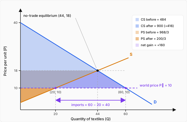
Concretely: left to itself, this country would trade 44 units of textiles among its own citizens at a price of 18 per unit. This pair of numbers, $(Q^*, P^*) = (44, 18)$, is the benchmark everything else gets measured against — it is the "Ann catches her own fish" scenario for this country.

Opening trade at a world price of 10

Now open the border, with the world offering textiles at $P_w = 10$. Since $10 < 18$, the decision rule says the country imports — the world is undercutting the domestic do-it-yourself price. But how much does it import? That is two separate questions: how much do domestic buyers want at the new, lower price, and how much are domestic mills still willing to produce at it?

Domestic quantity demanded at $P = 10$:

Domestic quantity supplied at $P = 10$:

At the cheaper world price, domestic buyers want 60 units — more than the 44 they bought before, because price falling moves them down along their demand curve. Domestic mills, facing a lower price that no longer covers their costs on the more expensive units, cut back to 20 units — moving down along their supply curve. Neither number involves any trade flow yet; they are just the domestic demand and supply curves evaluated at the fixed world price.

The gap between the two is exactly what must come from abroad:

Put plainly: the country consumes 60 units, makes 20 of them itself, and the remaining 40 arrive on those container ships. Imports are not a separate decision — they are simply the difference between what the country wants at the world price and what it still chooses to produce at the world price.

Winners, losers, and the net gain

Now the real question: who is better off, who is worse off, and by how much? The tools are exactly the consumer-surplus and producer-surplus measures used earlier — consumer surplus is the area under the demand curve above the price actually paid, and producer surplus is the area above the supply curve below the price received. Two facts about these particular curves make the areas easy. The demand curve $Q_d = 80 - 2P$ hits the price axis where $Q_d = 0$, namely $P = 40$, so inverse demand is $P = 40 - Q/2$. The supply curve $Q_s = -10 + 3P$ starts where $Q_s = 0$, namely $P = 10/3$, so inverse supply is $P = (Q + 10)/3$. Every surplus below is therefore an ordinary triangle, computable by hand.

Before trade — at the no-trade equilibrium $P^* = 18$, $Q^* = 44$:

Read that as: before trade, buyers enjoyed 484 of surplus — the bargain they got from paying 18 for units many of them valued at up to 40 — and the mills enjoyed about 322.67 of surplus — the profit margin they earned over their costs on each of the 44 units.

After trade — at the world price $P_w = 10$, with domestic buyers purchasing 60 and domestic mills producing 20:

Note carefully what goes into each: consumer surplus is measured on the full 60 units domestic buyers consume (including the imported ones — a bargain is a bargain wherever the shirt was sewn), while producer surplus is measured only on the 20 units domestic mills still produce.

Now take the differences, explicitly:

Consumers gain 416 from the cheaper price, and domestic producers lose 256 as the price falls out from under them. The evening-news stories were both true at once — shoppers genuinely are better off, and the mills genuinely are worse off. But the gains and losses are not equal. Add them:

Total surplus — consumer plus producer, counting only the home side of the border — rises by exactly 160, even though one domestic group is hurt. Equivalently, total surplus goes from $484 + \tfrac{968}{3} = \tfrac{2420}{3} \approx 806.67$ before trade to $900 + \tfrac{200}{3} = \tfrac{2900}{3} \approx 966.67$ after, and $\tfrac{2900}{3} - \tfrac{2420}{3} = \tfrac{480}{3} = 160$. Same number, computed a second way.

A third check pins down where those 160 come from geometrically, and it is worth doing because it shows the gain is real and not an accounting trick. Of the 416 consumers gain, most is just a transfer: 256 of it is surplus that used to belong to the mills and now belongs to shoppers, because the same units are bought 8 cheaper. That part is a reshuffling, not a net gain. The genuinely new surplus is the remaining $416 - 256 = 160$, and it splits into two triangles. First, new consumption: buyers purchase $60 - 44 = 16$ extra units they did not buy before, each worth more to them than the 10 they pay — a triangle of area $\tfrac12 \times 16 \times (18 - 10) = 64$. Second, freed resources: the mills stop producing $44 - 20 = 24$ units whose domestic cost (read off the supply curve, between 10 and 18) exceeded the world price of 10 — the country now gets those units cheaper from abroad, a saving of $\tfrac12 \times 24 \times (18 - 10) = 96$. And $64 + 96 = 160$, matching the algebraic answer to the unit. The upshot: trade creates value in two ways at once — it lets the country consume more of the good than it ever could cheaply make, and it stops the country from wasting expensive domestic effort on units the world will sell it for less.

Why this is comparative advantage all over again

Step back from the numbers and notice what the supply curve has been quietly telling you the whole time. Each point on it is the domestic opportunity cost of one more unit of textiles — the value of the labor, machines, and cotton that unit ties up, measured by what else those resources could have done. The units the mills stopped producing after trade, units 20 through 44, had domestic costs between 10 and 18. The world was offering those same units at 10. Buying them from the world instead of making them at home is precisely Ann's rule — trade for a good whenever the deal beats your own opportunity cost — applied at the scale of a whole country. The country imports textiles for exactly the same reason Ann traded for fish: not because it couldn't make them, but because making them cost more than trading for them. And the two triangles of new surplus are the country-scale version of the extra apples and fish that appeared when Ann and Bob swapped their hours — the value that appears when production is rearranged away from expensive sources and toward cheap ones. Comparative advantage was never really about two people on an island; the island was just the smallest stage on which the argument could be checked by hand.

Worked example

Where this leads

Look back at the long chain this topic closes. Scarcity forced trade-offs; comparative advantage said who should produce what; supply and demand showed how prices coordinate strangers; consumer and producer surplus turned those crossings into measurable value; and now, with a single horizontal line drawn across that machinery, the same tools have told us not just that countries gain from trade but exactly how much, and exactly whose pocket the gains come out of. It is worth noticing, though, how much has been quietly assumed all along: every market so far has been perfectly competitive, with many small buyers and sellers, no one powerful enough to set a price, no costs spilling onto bystanders, and everyone knowing exactly what they are buying. Real economies violate every one of those conditions, somewhere, and each violation breaks a different piece of the machinery built so far. The horizons ahead for this track are precisely those breakdowns: how individual consumers actually choose, what happens when markets are dominated by one firm or a few, and what to make of the cases — pollution, monopoly, hidden information — where the neat conclusion that markets maximize total surplus no longer holds. The tools you have now are the benchmark; everything next is about what happens when the benchmark bends.