Consumer Surplus, Producer Surplus, and Market Efficiency

Here's a small, happy moment you've almost certainly had. You walk up to a stall at the farmers' market wanting a basket of fresh wheat berries for the week's baking, and you've privately decided you'd go as high as $18 for it. The sign says $12. You hand over the money and walk away feeling oddly richer than the receipt justifies — because you are. You valued the basket at $18 and got it for $12; the $6 gap is a real gain, just not one that shows up in any cash register. The stall owner has her own version of the same feeling. Between feed, fuel, and her time, she'd have been willing to sell that basket for as little as $9 and still come out fine. Selling it at $12 leaves her $3 better off than her own private floor. Nothing about the price changed for anyone else in the market, yet both of you quietly captured a slice of value that nobody charged anyone for.

These two private numbers have names. The most a particular buyer is genuinely willing to pay for a good is her willingness to pay — not what she hopes to pay, but the price at which she'd be exactly indifferent between buying and walking away. The least a particular seller is genuinely willing to accept is his cost to produce — the number at which selling barely beats not selling. Every buyer in a market has her own willingness to pay, every seller his own cost, and they differ from person to person: the baker who needs wheat urgently will pay more than the hobbyist, and the efficient farm down the road can accept less than the one on the hillside.

Make it concrete with three imaginary buyers at our wheat market: Martha would pay up to $20 for a bushel, Luis up to $15, and Dana up to $11. If the going price is $12, Martha buys and pockets a personal gain of $20 - $12 = $8; Luis buys and gains $15 - $12 = $3; Dana looks at the price, compares it to her $11, and walks away with nothing gained and nothing lost. The total gain on the buyers' side that week is $8 + $3 = $11, and it came entirely from counting each person's private number against the actual price. That per-person difference — willingness to pay minus price actually paid, for everyone who actually buys — is what economists call consumer surplus. The mirror-image difference on the selling side — price received minus cost, for everyone who actually sells — is producer surplus.

Counting person by person works beautifully for three buyers. It becomes impossible for a real market with thousands of them, and that's exactly where the demand and supply curves from the last topic turn out to be hiding a gift: those curves are, in a precise sense, already the sorted list of everyone's private numbers. If that's true, then adding up all the individual gains should be the same as measuring a certain area between the curves — something one integral can do in a line.

That raises the deeper question this topic is really about. The wheat market we've been working with — demand $Q_d = 100 - 4P$ , supply $Q_s = -20 + 6P$ — settles on its own at price $P^* = 12$ and quantity $Q^* = 52$ . We now know how to measure the total gain that outcome creates. But is $Q^* = 52$ actually the best this market can do? Could some well-meaning organizer shuffle who trades with whom, or push a few more bushels through, and make the total gain bigger? The answer turns out to be a genuine theorem, provable with nothing more than the integral and one derivative, and it's the reason economists say competitive markets are "efficient."

Reading the curves vertically: what they actually stand for

Before any area gets computed, it pays to be exact about what the two curves mean, because the whole argument rests on it. In the supply-and-demand topic we wrote the wheat market as quantities that respond to price: $Q_d = 100 - 4P$ and $Q_s = -20 + 6P$ . For everything that follows, flip them around and write price as a function of quantity:

P = 25 - \tfrac{1}{4}Q \qquad \text{(inverse demand)}, \qquad\qquad P = \frac{20 + Q}{6} \qquad \text{(inverse supply)}.

Read the curve this way: the inverse demand curve tells you, at any quantity $Q$ , the willingness to pay of the marginal buyer — the person who is just barely willing to buy the $Q$ -th bushel. Check it at the start: at $Q = 0$ it says $P = 25$ , meaning the single most eager buyer in the whole market values a bushel at $25, and nobody values it higher. As $Q$ grows, the curve slides down through the less eager buyers: the $40$ th bushel goes to someone who values it at $25 - \tfrac{40}{4} = 15$ , and the $52$ nd at exactly $25 - \tfrac{52}{4} = 12$ . The inverse supply curve is the same idea on the other side: at each quantity it names the cost of the marginal seller — at $Q = 0$ the cheapest producer in the market can supply a bushel at a cost of $ $\tfrac{20}{6} = \tfrac{10}{3} \approx 3.33$ , and the $52$ nd bushel costs its producer exactly $\tfrac{20 + 52}{6} = 12$ .

This is what justifies everything below. Think of the buyers lined up in a row, sorted from most eager to least, each one a thin slice of width $1$ bushel with height equal to their own willingness to pay. Adding up "willingness to pay minus price" for every buyer is adding up the heights of those slices — and adding up infinitely many infinitely thin slices under a curve is precisely what a definite integral is. The area under the inverse demand curve, down to the price line, isn't a trick or an approximation: it is the sum of the individual gains, just counted smoothly instead of person by person. Same story for sellers, with the area above the inverse supply curve.

Consumer surplus, computed honestly

Consumer surplus is the total willingness to pay of everyone who buys, minus what they actually pay. Total willingness to pay for the first $Q^*$ bushels is the area under inverse demand from $0$ to $Q^*$ ; what buyers actually pay is the rectangle $P^* Q^*$ . With $P^* = 12$ and $Q^* = 52$ :

CS = \int_0^{52} \left(25 - \tfrac{1}{4}Q\right) dQ \;-\; P^* Q^*.

In plain words: add up every buyer's private valuation from the most eager down to the 52nd, then subtract the $12 \times 52$ dollars that actually changed hands. Carry out the integral:

\int_0^{52}\left(25 - \tfrac{1}{4}Q\right) dQ = \left[25Q - \tfrac{1}{8}Q^2\right]_0^{52} = 25(52) - \tfrac{1}{8}(52)^2 = 1300 - \frac{2704}{8} = 1300 - 338 = 962.

So buyers collectively valued those 52 thousand bushels at $962 thousand, while paying $P^* Q^* = 12 \times 52 = 624$ :

CS = 962 - 624 = 338 \text{ thousand dollars}.

Concretely: the wheat buyers as a group walk away each week with $338 thousand of value they would have paid but didn't have to — Martha's $8 and Luis's $3, extended smoothly across hundreds of buyers.

Because inverse demand here is a straight line, there's a completely independent way to get the same number: plain geometry. The surplus region is a triangle whose base runs from $Q = 0$ to $Q = 52$ and whose height is the gap between demand's vertical intercept, $P = 25$ , and the price, $P = 12$ :

CS = \tfrac{1}{2} \times \text{base} \times \text{height} = \tfrac{1}{2} \times 52 \times (25 - 12) = \tfrac{1}{2} \times 52 \times 13 = 338.

The calculus and the elementary-school triangle formula agree exactly — 338 either way — which is the kind of cross-check worth insisting on every time: if two honest routes to the same quantity disagreed, at least one of them would be lying.

Producer surplus, same treatment

Producer surplus is what sellers actually receive, minus the total cost of producing what they sold. Total cost of the first 52 thousand bushels is the area under the inverse supply curve — sum each marginal seller's cost, from the cheapest up to the 52nd — and total revenue is the same rectangle $P^* Q^* = 624$ :

PS = P^* Q^* - \int_0^{52} \frac{20 + Q}{6}\, dQ.

Put plainly: take the $624 thousand that came in, and subtract what it genuinely cost to grow those 52 thousand bushels, seller by seller, cheapest first. The integral:

\int_0^{52}\frac{20+Q}{6}\,dQ = \frac{1}{6}\left[20Q + \tfrac{1}{2}Q^2\right]_0^{52} = \frac{1}{6}\left(20(52) + \tfrac{1}{2}(2704)\right) = \frac{1}{6}(1040 + 1352) = \frac{2392}{6} = \frac{1196}{3}.

So total production cost was $ $\tfrac{1196}{3} \approx 398.67$ , and

PS = 624 - \frac{1196}{3} = \frac{1872 - 1196}{3} = \frac{676}{3} \approx 225.33 \text{ thousand dollars}.

The wheat farmers as a group earn about $225.33 thousand per week above what they'd have been willing to sell for. Cross-check with the triangle formula — this region has base 52 and height equal to the gap between the price $12$ and supply's vertical intercept $\tfrac{10}{3}$ :

PS = \tfrac{1}{2} \times 52 \times \left(12 - \tfrac{10}{3}\right) = \tfrac{1}{2} \times 52 \times \frac{26}{3} = \frac{676}{3} \approx 225.33. \quad\checkmark

A supply-and-demand chart of the wheat market with quantity in thousands of bushels per week (0–104) on the horizontal axis and price in dollars per bushel (0–26) on the vertical axis. A downward-sloping blue line labeled "Demand: P = 25 − Q/4" runs from (0, 25) to (100, 0); an upward-sloping orange line labeled "Supply: P = (20 + Q)/6" starts from (0, 10/3 ≈ 3.33). The lines cross at the equilibrium point (52, 12), marked with a dot and dashed gray guide lines to both axes. The triangle above the price line and below demand, with vertices (0, 12), (0, 25), and (52, 12), is shaded translucent blue and labeled "Consumer surplus = $338 thousand." The triangle below the price line and above supply, with vertices (0, 12), (0, 10/3), and (52, 12), is shaded translucent orange and labeled "Producer surplus = 676/3 ≈ $225 thousand." — Consumer and producer surplus in the wheat market at the competitive equilibrium P* = 12, Q* = 52: the blue triangle between the demand curve and the price is the buyers' $338 thousand; the orange triangle between the price and the supply curve is the sellers' roughly $225 thousand.

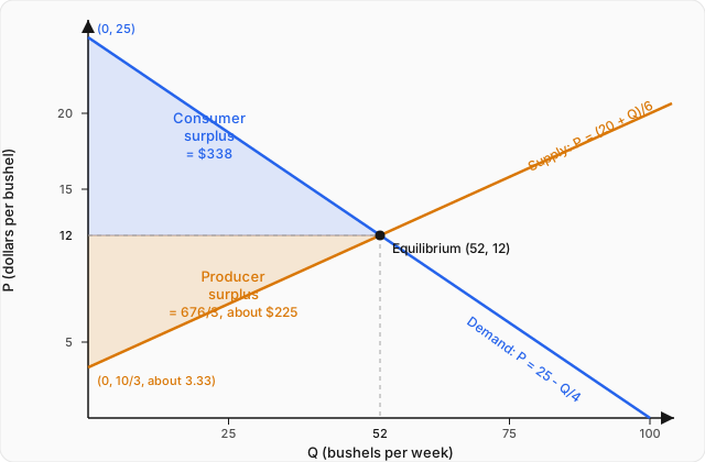
Total surplus — and a proof that equilibrium maximizes it

Total surplus is simply both groups' gains added together:

TS = CS + PS = 338 + \frac{676}{3} = \frac{1690}{3} \approx 563.33 \text{ thousand dollars per week}.

The upshot: this market, left alone, manufactures about $563 thousand of pure mutual gain every week — value that exists only because the trades happened. Now the promised theorem. Consider forcing the market to trade some other quantity $Q$ instead — always pairing the most eager buyers with the cheapest sellers, since any other pairing would only do worse. Each unit $q$ traded contributes a gain equal to the gap between what that unit's buyer values it at and what it costs its seller:

TS(Q) = \int_0^{Q} \left[\left(25 - \tfrac{1}{4}q\right) - \frac{20 + q}{6}\right] dq = \int_0^{Q}\left(\frac{65}{3} - \frac{5}{12}q\right) dq = \frac{65}{3}Q - \frac{5}{24}Q^2.

What that means: total gain is the accumulated area between the two curves — every bushel adds the vertical gap between what it's worth to its buyer and what it costs its seller. Sanity-check the formula at the equilibrium quantity: $TS(52) = \tfrac{65}{3}(52) - \tfrac{5}{24}(2704) = \tfrac{3380}{3} - \tfrac{1690}{3} = \tfrac{1690}{3}$ — exactly the $CS + PS$ we just computed two other ways, so the formula is consistent with everything above.

Now ask calculus where this function peaks. Differentiate with respect to $Q$ — by the fundamental theorem of calculus, the derivative of the integral is just the integrand evaluated at the endpoint — and set it to zero:

TS'(Q) = \frac{65}{3} - \frac{5}{12}Q = 0 \quad\Longrightarrow\quad Q = \frac{65}{3} \cdot \frac{12}{5} = 52.

The only candidate is $Q = 52$ — precisely the competitive equilibrium quantity, not approximately but exactly. And it really is a maximum, not a minimum or an inflection: $TS''(Q) = -\tfrac{5}{12} < 0$ everywhere, so the curve bends downward throughout.

The calculus has a plain-words reading worth saying out loud, because it's the real reason markets are efficient. $TS'(Q)$ is the gap between the curves: inverse demand minus inverse supply. For $Q < 52$ , the gap is positive — the marginal buyer values the next bushel more than it would cost the marginal seller to grow it, so every unit not traded below 52 is mutual gain being left on the table: there's a buyer standing above the supply curve and a seller below the demand curve who never got matched. For $Q > 52$ , the gap flips negative — the marginal buyer values those extra bushels less than they cost to produce, so forcing them through actively destroys value. The market's invisible hand, pushing price until quantity demanded equals quantity supplied, stops trading at exactly the quantity where the marginal gap hits zero — and, as the derivative just proved, that is exactly where total surplus peaks. Efficiency isn't a slogan about markets; it's a theorem about this integral.

Worked example

Suppose a quota restricts the wheat market to $Q = 40$ thousand bushels per week, with the 40 cheapest sellers supplying the 40 most eager buyers and the price settling at the marginal buyer's willingness to pay. Recompute consumer surplus, producer surplus, and total surplus, and quantify the loss relative to the free market.

Step 1 — the price under the quota. At $Q = 40$ , inverse demand gives the marginal buyer's willingness to pay:

P = 25 - \tfrac{1}{4}(40) = 15 \text{ dollars}.

Step 2 — consumer surplus. Buyers now pay 15 for 40 thousand bushels:

CS = \int_0^{40}\left(25 - \tfrac{1}{4}Q\right)dQ - 15(40) = \left[25Q - \tfrac{1}{8}Q^2\right]_0^{40} - 600 = (1000 - 200) - 600 = 200.

(Triangle check: $\tfrac12 \times 40 \times (25 - 15) = 200$ .) Buyers lose $338 - 200 = 138$ — from both paying more and buying less.

Step 3 — producer surplus. Sellers receive 15 per bushel; costs are the area under inverse supply up to 40:

PS = 15(40) - \int_0^{40}\frac{20+Q}{6}\,dQ = 600 - \frac{1}{6}\left[20Q + \tfrac12 Q^2\right]_0^{40} = 600 - \frac{1}{6}(800 + 800) = 600 - \frac{800}{3} = \frac{1000}{3} \approx 333.33.

Interestingly, sellers gain $108$ — the higher price more than compensates them for selling fewer bushels — which hints at why sellers sometimes lobby for exactly such restrictions.

Step 4 — total surplus and the loss.

TS = 200 + \frac{1000}{3} = \frac{1600}{3} \approx 533.33, \qquad \text{loss} = \frac{1690}{3} - \frac{1600}{3} = \frac{90}{3} = 30 \text{ dollars per week}.

As the theorem promised, total surplus at $Q = 40$ is strictly below the free-market $\tfrac{1690}{3}$ . The $30 loss matches the closed-form $TS(Q)$ directly: $TS(52) - TS(40) = \tfrac{1690}{3} - \left(\tfrac{65}{3}(40) - \tfrac{5}{24}(1600)\right) = \tfrac{1690}{3} - \tfrac{1600}{3} = 30$ . It also has a clean geometric meaning: it's the triangle between the two curves from $Q = 40$ to $Q = 52$ , i.e. $\tfrac12 \times (52 - 40) \times (15 - 10) = \tfrac12 \times 12 \times 5 = 30$ — the mutual gains on the 12 thousand bushels that never got traded, from buyers who valued them between $12 and $15 and sellers who'd have grown them for between $10 and $12. Note that the quota didn't just move surplus around — buyers lost 138 while sellers gained only 108, and the missing 30 simply vanished.

Where this leads

We now have a measuring instrument: consumer surplus, producer surplus, and their sum tell us exactly how much a market outcome is worth to the people in it, and the efficiency theorem tells us the unregulated competitive outcome scores as high as any arrangement possibly can. But real markets are rarely left entirely alone — governments tax them. A tax wedges a gap between what buyers pay and what sellers receive, shrinks the quantity traded, and hands some of the surplus to the treasury. The surplus machinery built here is precisely sharp enough to answer the hard question about that: how much of the lost surplus is merely transferred to the government, and how much disappears entirely, captured by no one — the deadweight loss. That's the subject of the next topic: The Costs of Taxation: Deadweight Loss.