Elasticity and Its Applications

Ask a room full of wheat farmers whether they're hoping for good weather this year, and every hand will go up. Now tell them something that sounds like a riddle: there are years when a bad harvest — a drought or a frost that wipes out a chunk of the whole country's wheat crop — leaves farmers, taken as a group, richer than a good harvest does. Not the individual farmer whose own field was destroyed; that farmer is plainly worse off. But add up every farmer's earnings in a bad-harvest year, and the total can come out higher than in a year when the weather was kind and the silos overflowed. Less wheat to sell, yet more money earned. That should be impossible — and the fact that it isn't tells you something deep about how markets work.

The tools from the last topic get you partway to the answer. A bad harvest shifts the supply curve to the left: at every price, there is less wheat available. With demand unchanged, the market slides up along the demand curve to a new equilibrium — the price rises, and the quantity sold falls. So far, so good. But notice what the supply-and-demand machinery does not tell you. It tells you which direction price and quantity move; it says nothing about how much they move. And "how much" is exactly what settles the riddle, because the farmers' total earnings — what economists call total revenue, the price multiplied by the quantity actually sold — are caught between two opposing effects: each bushel sells for more, but fewer bushels get sold.

Which effect wins? The natural first guess is that it's a coin flip, depending on the details of the weather. The truth is much better than that. It turns out the answer is decided entirely by one measurable property of the demand curve: not just which way it slopes, but how strongly buyers respond when the price changes. If buyers barely cut back when wheat gets expensive, the price effect dominates and revenue rises; if buyers flee to substitutes at the first hint of a price increase, the quantity effect dominates and revenue falls. Economists call this responsiveness elasticity, and it is arguably the single most useful number in all of applied microeconomics.

There is one subtlety to clear away before any of this can be made precise, and it's about units. "How strongly buyers respond" can't be measured in raw units — bushels per dollar — because then the answer would depend on arbitrary choices: measure wheat in bushels or in tons, price it in dollars or in cents, and you get different numbers for the same underlying behavior. Worse, raw-unit numbers can't be compared across markets: "4 bushels per dollar" for wheat and "2 barrels per dollar" for oil tell you nothing about which market is more responsive. The fix, as we'll see, is to measure everything in percentages, so the units cancel out entirely.

So here is the precise question this topic answers, using the same wheat market from the supply-and-demand topic and nothing beyond arithmetic and one rule of calculus: how do you define and compute a units-free measure of responsiveness, and how does that single number rigorously determine what happens to total revenue when supply shifts — including the bad-harvest paradox?

What elasticity actually measures

Elasticity is a ratio of percentage changes. The price elasticity of demand asks: if the price of a good rises by one percent, by what percent does the quantity demanded fall? Because quantity demanded moves opposite to price, this number comes out negative, and economists usually compare elasticities by absolute value. The classification has three cases, worth naming before deriving anything:

Elastic demand, $|\varepsilon| > 1$ : quantity responds more than proportionally — a 1% price rise cuts quantity demanded by more than 1%.
Unit elastic demand, $|\varepsilon| = 1$ : quantity responds exactly proportionally.
Inelastic demand, $|\varepsilon| < 1$ : quantity responds less than proportionally — buyers barely budge.

Put plainly: elasticity measures how skittish the other side of the market is. Goods with close substitutes (one brand of coffee versus another) tend to have elastic demand; goods with few substitutes and no room to adjust (insulin, gasoline in the short run) tend to have inelastic demand. The same construction works for the supply curve — how strongly producers respond — and for other kinds of changes entirely, like income, as the worked example at the end will show.

The point elasticity of demand

Back to the wheat market. From the supply-and-demand topic, demand and supply are

Q_d = 100 - 4P, \qquad Q_s = -20 + 6P,

with equilibrium found by setting them equal: $100 - 4P = -20 + 6P \Rightarrow 120 = 10P \Rightarrow P^* = 12$ dollars per bushel and $Q^* = 100 - 4(12) = 52$ thousand bushels. Total revenue at equilibrium is $TR = 12 \times 52 = 624$ — hold that number, because the whole bad-harvest story will be judged against it.

Now turn the verbal definition into a formula. A percentage change is a change divided by a starting level, so for a tiny price change $dP$ and the resulting tiny quantity change $dQ$ :

\varepsilon_d = \frac{dQ / Q}{dP / P} = \frac{dQ}{dP}\cdot\frac{P}{Q}.

In plain words: elasticity is the slope of the demand curve, $dQ/dP$ , rescaled by where you currently are on it, $P/Q$ . The rescaling is what makes the units cancel — bushels cancel bushels, dollars cancel dollars — so the same formula works for wheat, oil, or concert tickets.

Apply it. For $Q_d = 100 - 4P$ , the derivative is $dQ/dP = -4$ , a constant, since the demand curve is a straight line. At the equilibrium point $(P^*, Q^*) = (12, 52)$ :

\varepsilon_d = (-4)\cdot\frac{12}{52} = -\frac{48}{52} = -\frac{12}{13} \approx -0.92.

Concretely: near the equilibrium, a 1% increase in the price of wheat reduces the quantity demanded by about 0.92% — slightly less than proportionally. Since $|\varepsilon_d| = 12/13 < 1$ , demand is inelastic at the equilibrium. That single fact will turn out to be the entire explanation of the bad-harvest paradox.

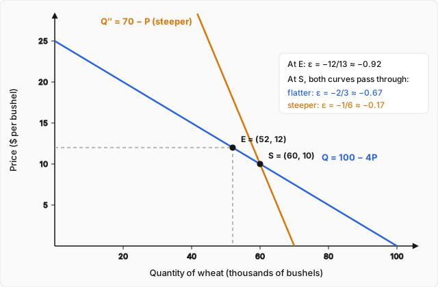
One warning before moving on: elasticity is not the same thing as slope, and confusing them is the most common mistake in this whole subject. The slope of this demand curve is $-4$ everywhere, but the elasticity changes from point to point because the $P/Q$ factor changes. At $P = 10$ , $Q = 60$ : $\varepsilon_d = -4 \cdot \tfrac{10}{60} = -\tfrac23 \approx -0.67$ . At $P = 20$ , $Q = 20$ : $\varepsilon_d = -4 \cdot \tfrac{20}{20} = -4$ . In plain words, the same straight line is inelastic at low prices and elastic at high prices — steepness alone doesn't determine responsiveness, which is exactly why elasticity had to be defined as a separate object.

From a point to an arc: the midpoint formula

The derivative formula answers a question about an infinitesimal nudge. Real price changes are lumpy — wheat actually jumping from $P = 10$ to $P = 14$ , say. On this demand curve, quantity falls from $Q(10) = 60$ to $Q(14) = 44$ , so $\Delta Q = -16$ against $\Delta P = 4$ . To convert these into percentages you need a base, and here's the catch: using the starting point gives $(-16/60)/(4/10) = -\tfrac23 \approx -0.67$ , while using the ending point gives $(-16/44)/(4/14) = -\tfrac{14}{11} \approx -1.27$ . Same price change, two very different answers, depending on an arbitrary choice of direction.

The standard fix is the midpoint (or arc) convention: use the average of the two endpoints as the base for both percentages. With $\bar P = (10+14)/2 = 12$ and $\bar Q = (60+44)/2 = 52$ :

\varepsilon_{\text{arc}} = \frac{\Delta Q / \bar Q}{\Delta P / \bar P} = \frac{\Delta Q}{\Delta P}\cdot\frac{\bar P}{\bar Q} = \frac{-16}{4}\cdot\frac{12}{52} = -\frac{12}{13} \approx -0.92.

Measured symmetrically over this whole move, demand responds a little less than proportionally — the same inelastic verdict as before.

Now compare with the point formula evaluated at the midpoint $(12, 52)$ : $\varepsilon_d = -4 \cdot \tfrac{12}{52} = -\tfrac{12}{13}$ . The two agree exactly, and it's worth being honest about why. For a straight-line demand curve, $\Delta Q/\Delta P$ between any two points equals the derivative $dQ/dP$ exactly, and the midpoint averages $\bar P, \bar Q$ are exactly the coordinates of the midpoint — so the arc formula and the point formula at the midpoint are the same computation in disguise. On a curved demand curve neither shortcut holds: the chord slope only approximates the derivative, and the arc answer comes out close to, but not identical to, the point elasticity at the midpoint. What genuinely differs even here is the point elasticity at the endpoints: the arc value $-0.92$ lies strictly between $-\tfrac23$ at $P=10$ and $-\tfrac{14}{11}$ at $P=14$ , behaving like what it is — an average of the responsiveness over the whole segment. The difference: point elasticity answers "how responsive is demand right here," while arc elasticity answers "how responsive was demand over this whole move," and for a straight-line curve the arc answer lands exactly on the point answer at the midpoint.

A chart with quantity of wheat in thousands of bushels on the horizontal axis, running 0 to 100, and price in dollars per bushel on the vertical axis, running 0 to 25. Two straight downward-sloping demand curves cross at a shared point (60, 10): a flatter blue line for Q = 100 − 4P, running from (0, 25) on the price axis to (100, 0) on the quantity axis, and a steeper orange line for Q = 70 − P, entering the top edge of the chart near price 29 and reaching the quantity axis at 70. A black dot labeled E marks the market equilibrium (52, 12) on the blue curve, with dashed gray guide lines dropping to the quantity axis and running left to the price axis; a legend notes its elasticity is −12/13, about −0.92. A second black dot labeled S marks the shared crossing point (60, 10), where the legend notes the flatter blue curve has elasticity −2/3 while the steeper orange curve has −1/6, showing that at one and the same point a flatter curve is more elastic. — Two demand curves through the shared point S = (60, 10). The flatter curve, Qd = 100 - 4P, has elasticity -2/3 there; the steeper hypothetical curve, Qd' = 70 - P, has elasticity -1/6 at the same point. Flatter means more elastic: at the same price and quantity, the curve whose quantity responds more strongly to a price change is the more elastic one. The market equilibrium E = (52, 12) sits on the flatter curve, where the elasticity is -12/13, about -0.92.

The price elasticity of supply

The identical construction works on the producers' side, asking how strongly the quantity supplied responds to price. Starting from the percentage definition and rearranging exactly as before:

\varepsilon_s = \frac{dQ_s}{dP}\cdot\frac{P}{Q}.

For $Q_s = -20 + 6P$ , the derivative is $dQ_s/dP = 6$ , so at the equilibrium $(12, 52)$ :

\varepsilon_s = 6\cdot\frac{12}{52} = \frac{72}{52} = \frac{18}{13} \approx 1.38.

Read that as: a 1% higher price calls forth about 1.38% more wheat supplied — producers respond more than proportionally, so supply is elastic at the equilibrium. Note the sign is positive, because supply slopes up; the absolute-value convention is only needed for demand. Together the two numbers say something memorable about this market: at the equilibrium, buyers are the sluggish side and sellers are the nimble side.

Why a bad harvest can raise farm revenue: the total revenue rule

Now the payoff. Total revenue, viewed as a function of price along the demand curve, is $TR(P) = P \cdot Q(P)$ . Differentiate with the product rule — and do it honestly, step by step:

\frac{d(TR)}{dP} = \frac{d}{dP}\left[P \cdot Q(P)\right] = Q(P) + P\,\frac{dQ}{dP}.

Unpacked: raising the price by a dollar has two effects — you earn a dollar more on every unit you still sell (the $Q$ term), but you lose the revenue on the units that no longer get bought (the $P\, dQ/dP$ term, which is negative). Factor out $Q$ and recognize the elasticity formula hiding inside:

\frac{d(TR)}{dP} = Q\left(1 + \frac{P}{Q}\cdot\frac{dQ}{dP}\right) = Q\left(1 + \varepsilon_d\right).

What that means: the direction revenue moves when price rises is decided entirely by whether $\varepsilon_d$ is above or below $-1$ . Since $Q > 0$ always, the sign of $d(TR)/dP$ is the sign of $1 + \varepsilon_d$ . This gives the total-revenue rule, now derived rather than asserted:

Inelastic demand ( $|\varepsilon_d| < 1$ , i.e. $\varepsilon_d > -1$ ): $d(TR)/dP > 0$ — raising the price raises revenue.
Elastic demand ( $|\varepsilon_d| > 1$ ): $d(TR)/dP < 0$ — raising the price lowers revenue.
Unit elastic ( $\varepsilon_d = -1$ ): $d(TR)/dP = 0$ — revenue is at its maximum, flat to first order.

Check the arithmetic a second way, the honest way. Along this demand curve, $TR(P) = P(100 - 4P) = 100P - 4P^2$ , so $d(TR)/dP = 100 - 8P$ . At the equilibrium price $P^* = 12$ : $100 - 8(12) = 4$ . And from the elasticity formula: $Q(1 + \varepsilon_d) = 52\left(1 - \tfrac{12}{13}\right) = 52 \cdot \tfrac{1}{13} = 4$ . The two computations agree exactly — revenue is increasing in price at the equilibrium, by 4 thousand dollars per dollar of price — and the direct formula also shows revenue peaks where $100 - 8P = 0$ , at $P = 12.5$ , exactly the price where $\varepsilon_d = -4 \cdot \tfrac{12.5}{50} = -1$ . In plain words, the revenue-maximizing price is precisely the price where demand turns from inelastic to elastic, just as the rule demands.

The bad-harvest paradox is now one short calculation away. Suppose drought shifts supply left to $Q_s' = -25 + 6P$ — five thousand fewer bushels available at every price. The new equilibrium solves $100 - 4P = -25 + 6P \Rightarrow 125 = 10P \Rightarrow P = 12.5$ , $Q = 100 - 4(12.5) = 50$ . Revenue before: $12 \times 52 = 624$ . Revenue after: $12.5 \times 50 = 625$ . Farmers collectively sell 2 thousand fewer bushels and still come out one thousand dollars ahead — because over this entire move demand stayed inelastic ( $|\varepsilon_d| \le 1$ from $P = 12$ up to $P = 12.5$ ), so every step up in price added more revenue on units still sold than it lost on units no longer bought, which is exactly what $d(TR)/dP = Q(1+\varepsilon_d) \ge 0$ says. The riddle from the opening is solved, with no hand-waving: when demand is inelastic, a leftward supply shift raises the price by a larger percentage than it reduces the quantity, and group revenue rises. And it carries its own caveat, visible in the derivation — this only works because the price was free to rise.

Worked example

A household's monthly income rises from $2,000 to $2,200, and its monthly purchases of wheat bread rise from 25 loaves to 26 loaves. (a) Compute the household's income elasticity of demand for bread using the midpoint convention. (b) Is bread a necessity or a luxury for this household?

Step 1 — percentage changes, midpoint bases. The quantity change is $\Delta Q = 1$ loaf against an average of $\bar Q = (25 + 26)/2 = 25.5$ , and the income change is $\Delta I = 200$ against an average of $\bar I = (2000 + 2200)/2 = 2100$ :

\frac{\Delta Q}{\bar Q} = \frac{1}{25.5} \approx 0.0392, \qquad \frac{\Delta I}{\bar I} = \frac{200}{2100} \approx 0.0952.

Purchases rose about 3.9% while income rose about 9.5%.

Step 2 — divide the percentages. Income elasticity is defined exactly like price elasticity, with income in place of price:

\varepsilon_I = \frac{\Delta Q / \bar Q}{\Delta I / \bar I} = \frac{0.0392}{0.0952} \approx 0.41.

Using the simpler starting-value percentages instead gives $4\% / 10\% = 0.40$ — nearly identical, as expected for small changes. Each 1% rise in income raises bread purchases by only about 0.4%.

Step 3 — classify. The sign is positive, so bread is a normal good: demand rises with income rather than falling (an inferior good, like instant noodles for many households, would have $\varepsilon_I < 0$ ). But $0 < \varepsilon_I < 1$ , so bread is a necessity — demand grows slower than income. A luxury would show $\varepsilon_I > 1$ , purchases growing faster than income. The household gets 10% richer and buys only about 4% more bread: it was already buying most of the bread it wanted.

Where this leads

Elasticity answered the "how much" question that supply and demand left open, and in doing so it quietly became the deciding variable in every revenue question — including the strange case of farmers profiting, as a group, from their own misfortune. But notice the one assumption that entire argument leaned on: when supply shifted left, the price was allowed to rise, carrying the market to its new equilibrium. Governments don't always allow that. After a bad harvest, a legislature under pressure from angry consumers may cap the price of bread; in other markets it may wedge a tax between what buyers pay and what sellers receive. What happens to the market then — who gains, who loses, and which side of the market really ends up paying — turns out to depend, once again, on exactly the elasticities derived here. That is the subject of the next topic: Price Controls and the Economics of Taxes.