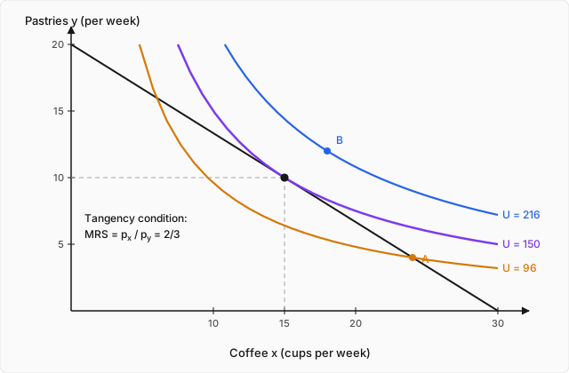
Consumer Choice and Utility Maximization

Nadia keeps 120 dollars a week for the bakery on Harbor Falls' main street. Coffee is 4 dollars a cup, pastries are 6. She has never written down an equation about this in her life, and yet if you follow her for a month you find her buying, almost exactly, fifteen coffees and ten pastries a week. Not twenty and seven. Not six and sixteen. The same corner of the same two-dimensional space, week after week.

That regularity should bother you slightly, because nothing has forced it. She could afford thirty coffees and no pastries. She could afford twenty pastries and no coffee. She could afford any of the infinitely many mixtures in between, and every one of them uses the full 120 dollars just as completely as the bundle she actually picks. Whatever selects fifteen-and-ten out of that continuum is not the budget — the budget is indifferent between all of them.

And here is why it matters beyond one person's breakfast. Supply, Demand, and Market Equilibrium opened with a demand curve, $Q_d = 100 - 4P$ , and justified it in a sentence: at higher prices, buyers want less. Elasticity and Its Applications then built an entire apparatus on top of that curve — measuring its slope, classifying its responsiveness, deriving who bears a tax. Both topics used the demand curve. Neither derived it. Where does a demand curve come from? What is it a picture of?

This is the first university-level topic in this track, and it is where that question gets answered rather than deferred. Everything before this described markets from the outside — curves crossing, surpluses, wedges. From here we go underneath, to the person, and build the curve out of something more primitive: what she can afford, what she wants, and one piece of constrained optimization. The mathematics is calculus with several variables and a Lagrange multiplier. That is not a detour and it will not be apologized for — it is the only honest way to get the result, and the multiplier itself turns out to have an economic meaning so clean that it is worth the whole derivation on its own.

What you can afford: the budget constraint

Start with the part that involves no psychology at all. Write $x$ for cups of coffee per week and $y$ for pastries per week, with prices $p_x$ and $p_y$ and income $m$ . Nadia can buy any bundle $(x,y)$ that satisfies

p_x x + p_y y \le m,

and with her numbers, $4x + 6y \le 120$ . The set of bundles satisfying this is the budget set; its outer edge, where the inequality binds,

p_x x + p_y y = m,

is the budget line. Solve it for $y$ to see it as a graph:

y = \frac{m}{p_y} - \frac{p_x}{p_y}\,x = 20 - \frac{2}{3}x.

Three numbers in that line are worth naming, because every comparative-static result later in the topic is one of them moving.

The vertical intercept $m/p_y = 120/6 = 20$ is what she gets spending everything on pastries. The horizontal intercept $m/p_x = 120/4 = 30$ is everything on coffee. And the slope, $-p_x/p_y = -4/6 = -2/3$ , is the interesting one. It is not a statement about Nadia. It says: the market will trade you one more coffee in exchange for two-thirds of a pastry, and it will do so at that rate all day. Give up a pastry, free 6 dollars, buy one and a half coffees. The slope of the budget line is the market rate of exchange between the two goods — the opportunity cost of coffee measured in pastries, which is exactly the notion Opportunity Cost and the Production Possibilities Frontier built for production and which now reappears, unchanged, on the consumption side.

Notice what the slope does not contain: income. Divide the constraint by $p_y$ and $m$ appears only in the intercept. So the two kinds of change are cleanly separated:

Income changes. Double $m$ to 240 and the line becomes $y = 40 - \frac23 x$ : same slope, both intercepts doubled. The budget line shifts out parallel to itself. Nothing about relative scarcity changed; there is simply more of everything available.
A price change. Raise $p_x$ from 4 to 6 and the line becomes $y = 20 - x$ : the vertical intercept is untouched (spending everything on pastries is unaffected by the price of coffee), the horizontal intercept falls from 30 to 20, and the line pivots, getting steeper.

That asymmetry is the seed of something. A price change does two things at once — it shrinks the budget set, like a loss of income, and it tilts it, changing the exchange rate. Hold that thought; the closing section comes back to it, and it is the reason a whole separate topic exists.

One assumption is buried in writing the constraint with an equality. Why should Nadia spend all 120 dollars? Only because we are about to assume she always prefers more to less, so that leftover money is wasted utility. That assumption is called monotonicity, and it is one of four we now have to be explicit about.

What you want: preferences and indifference curves

The budget set says what is possible. To pick a point out of it we need to describe what Nadia wants, and the trick that makes this tractable is to describe preferences by ranking bundles rather than by measuring them. Write $(x_1,y_1) \succeq (x_2,y_2)$ to mean "she likes the first at least as well as the second." Four assumptions on that ranking do all the work:

Completeness. For any two bundles, either $A \succeq B$ or $B \succeq A$ (or both). She is never simply unable to compare. This buys you the existence of a best element — without it, an optimum might not be well defined at all.

Transitivity. If $A \succeq B$ and $B \succeq C$ then $A \succeq C$ . This buys you consistency, and it is less innocuous than it sounds: a consumer with intransitive preferences can be walked around a cycle of trades she accepts at every step and returned to where she started, minus a fee. Transitivity is what rules out that money pump.

Monotonicity. More is better: if a bundle has at least as much of both goods and strictly more of one, it is strictly preferred. This buys you two things — the budget constraint binds with equality, and indifference curves slope downward (give up some $x$ and you must be compensated with some $y$ to stay indifferent).

Convexity. Averages are at least as good as extremes: if $A \sim B$ , then the mixture $\tfrac12 A + \tfrac12 B$ is at least as good as either. This is the assumption that makes moderate bundles attractive — it is why Nadia buys some coffee and some pastries rather than going all-in on one. It is also, as we will prove below, the assumption that turns a point where calculus says "stationary" into a point where economics says "best."

Now represent the ranking by a utility function $U(x,y)$ chosen so that $U(A) \ge U(B)$ exactly when $A \succeq B$ . Crucially, only the ordering is meaningful. If $U$ represents Nadia's preferences then so does $U^3$ , or $\ln U$ , or $2U + 7$ — any strictly increasing transformation, because it reorders nothing. There is no unit of utility, no "utils per pastry" you could measure with an instrument. Anything we derive that depends on the level of $U$ is an artifact; anything that survives every monotonic transformation is real economics. We will use this fact twice, and get caught by it once.

For Nadia, take

U(x,y) = xy.

An indifference curve is a level set of $U$ — the collection of bundles she rates equally. Setting $xy = \bar U$ gives $y = \bar U / x$ , a hyperbola. Her observed bundle $(15,10)$ sits on $\bar U = 150$ . The bundle $(24,4)$ sits on $\bar U = 96$ , and $(18,12)$ on $\bar U = 216$ . Higher curves are better, by monotonicity, and no two curves cross — if they did, transitivity would fail on the spot, since the crossing bundle would be indifferent to points on both curves while those points are not indifferent to each other.

The marginal rate of substitution

The slope of an indifference curve is the single most important derivative in consumer theory, and it deserves to be derived rather than asserted. Take the defining equation of one curve,

U(x,y) = \bar U,

and totally differentiate both sides. The right side is a constant, so its differential is zero:

\frac{\partial U}{\partial x}\,dx + \frac{\partial U}{\partial y}\,dy = 0.

Solve for the slope:

\left.\frac{dy}{dx}\right|_{U = \bar U} = -\frac{\partial U/\partial x}{\partial U/\partial y} = -\frac{MU_x}{MU_y}.

The marginal rate of substitution is defined as the magnitude of that slope:

\boxed{\;MRS = \frac{\partial U/\partial x}{\partial U/\partial y} = \frac{MU_x}{MU_y}\;}

Read it as a willingness, not a technology: $MRS$ is the number of pastries Nadia would hand over for one more coffee and feel exactly as well off. It is her personal exchange rate, in the same units as the market's exchange rate $p_x/p_y$ , which is what will let us set them equal in a moment.

Notice immediately that the $MRS$ survives monotonic transformation. Replace $U$ by $g(U)$ with $g' > 0$ ; the chain rule gives $\partial g/\partial x = g'(U)\,MU_x$ and likewise for $y$ , and the common factor $g'(U)$ cancels in the ratio. The $MRS$ is real. The number $U(x,y)$ itself is not.

For $U = xy$ the partials are $MU_x = y$ and $MU_y = x$ , so

MRS(x,y) = \frac{y}{x}.

Evaluate it along the curve $\bar U = 150$ , where $y = 150/x$ , so $MRS = 150/x^2$ :

\begin{array}{r|rrrrr} x & 6 & 10 & 15 & 20 & 25 \\ \hline y = 150/x & 25 & 15 & 10 & 7.5 & 6 \\ MRS = y/x & 4.1\overline{6} & 1.5 & 0.6\overline{6} & 0.375 & 0.24 \end{array}

The $MRS$ falls as she moves right along the curve. This is diminishing marginal rate of substitution, and it is convexity in derivative form: when she has 6 coffees and 25 pastries, one more coffee is worth over four pastries to her; when she already has 25 coffees and 6 pastries, one more coffee is worth barely a quarter of a pastry. The good she is short of is the good she values at the margin.

The connection to convexity is exact rather than rhetorical. Differentiate the indifference curve $y(x) = \bar U/x$ twice: $y' = -\bar U/x^2$ and $y'' = 2\bar U/x^3 > 0$ . A curve with $y'' > 0$ lies above every one of its chords, which is precisely the statement that the average of two indifferent bundles is weakly preferred. Convex preferences, diminishing $MRS$ , and indifference curves bowed toward the origin are three descriptions of one fact.

The optimum, three ways

Now put the two halves together. Nadia wants to reach the highest indifference curve that the budget set allows.

First, geometrically. Suppose she is at an interior bundle on the budget line where $MRS \ne p_x/p_y$ — say $MRS > p_x/p_y$ . Her indifference curve through that point is steeper than the budget line, so the two curves cross rather than touch, which means part of the budget line pokes above her indifference curve. Any point on that part is affordable and strictly better. The same argument runs in reverse if $MRS < p_x/p_y$ . So at an interior optimum, crossing is impossible, and the only remaining possibility is tangency:

MRS = \frac{p_x}{p_y}.

In words, and this is the whole idea: the rate at which she is willing to trade equals the rate at which the market lets her trade. Whenever those two rates differ, there is a trade she wants that the market will give her.

Second, by arbitrage, with numbers. Take the bundle $(24,4)$ , which is on the budget line — $4(24) + 6(4) = 96 + 24 = 120$ — so it is affordable and uses every dollar. Its marginal utilities are $MU_x = y = 4$ and $MU_y = x = 24$ . Ask what one dollar buys on each side:

\frac{MU_x}{p_x} = \frac{4}{4} = 1, \qquad \frac{MU_y}{p_y} = \frac{24}{6} = 4.

A dollar spent on pastry delivers four times what a dollar spent on coffee delivers. So move dollars: give up 3 coffees, freeing 12 dollars, and buy 2 pastries. The new bundle is $(21,6)$ , still costing $84 + 36 = 120$ , and its utility is $21 \times 6 = 126$ — up from 96, for zero extra money. Repeat the reasoning at $(21,6)$ : $MU_x/p_x = 6/4 = 1.5$ and $MU_y/p_y = 21/6 = 3.5$ , still unequal, so keep going. The process only stops when

\frac{MU_x}{p_x} = \frac{MU_y}{p_y},

which is the tangency condition rearranged — divide through and $MU_x/MU_y = p_x/p_y$ is back. This form is worth memorizing in its own words: the last dollar spent on each good must buy the same marginal utility. If it did not, a dollar could be moved and something gained for nothing, and that is not what an optimum looks like.

Third, by Lagrange, which is the version that generalizes. Maximize $U(x,y)$ subject to $p_x x + p_y y = m$ . Form

\mathcal{L}(x,y,\lambda) = U(x,y) + \lambda\left(m - p_x x - p_y y\right),

and set the three partial derivatives to zero:

\frac{\partial \mathcal{L}}{\partial x} = \frac{\partial U}{\partial x} - \lambda p_x = 0, \qquad \frac{\partial \mathcal{L}}{\partial y} = \frac{\partial U}{\partial y} - \lambda p_y = 0, \qquad \frac{\partial \mathcal{L}}{\partial \lambda} = m - p_x x - p_y y = 0.

The first two rearrange to

\boxed{\;\frac{\partial U/\partial x}{p_x} = \frac{\partial U/\partial y}{p_y} = \lambda\;}

which is the equal-marginal-utility-per-dollar condition, now with a name for the common value. Dividing the first two equations instead of setting them equal gives $MU_x/MU_y = p_x/p_y$ , the tangency condition. The third equation is just the budget constraint, recovered for free — which is the whole reason the multiplier is introduced this way.

Solve for Nadia. With $U = xy$ : $y = \lambda p_x = 4\lambda$ and $x = \lambda p_y = 6\lambda$ . Substituting into the constraint,

4(6\lambda) + 6(4\lambda) = 120 \quad\Longrightarrow\quad 48\lambda = 120 \quad\Longrightarrow\quad \lambda = 2.5,

and therefore $x^* = 6(2.5) = 15$ and $y^* = 4(2.5) = 10$ . Fifteen coffees and ten pastries — the bundle we started the topic by observing. Check the tangency: $MRS(15,10) = 10/15 = 2/3$ , and $p_x/p_y = 4/6 = 2/3$ . ✓

What $\lambda$ means. The multiplier is not bookkeeping; it is the marginal utility of income. Prove it here rather than quoting it. Solve the problem for general $m$ : the same algebra gives $x^*= m/(2p_x)$ and $y^* = m/(2p_y)$ , so the maximized utility is

U^*(m) = x^* y^* = \frac{m}{2p_x}\cdot\frac{m}{2p_y} = \frac{m^2}{4 p_x p_y}.

Differentiate with respect to income:

\frac{dU^*}{dm} = \frac{2m}{4p_xp_y} = \frac{m}{2p_xp_y} = \frac{120}{2(4)(6)} = \frac{120}{48} = 2.5 = \lambda. \;\checkmark

So $\lambda$ answers "how much better off is she made by one more dollar?" — 2.5 units of $U$ per dollar, at these prices and this income. (This is the envelope theorem in its smallest possible case, and it is the same structure as the shadow prices that appear all over constrained optimization.)

And here is the place we get caught by the earlier warning. Utility levels are not meaningful, so $\lambda$ 's numerical value cannot be either. Replace $U = xy$ by $V = \ln x + \ln y$ , which represents identical preferences. The first-order conditions become $1/x = \lambda_V p_x$ and $1/y = \lambda_V p_y$ , giving $p_x x = p_y y = 1/\lambda_V$ , and with the budget, $\lambda_V = 2/m = 1/60$ . Same bundle $(15,10)$ — as it must be, since the preferences are the same — but $\lambda_V = 1/60$ , nothing like 2.5. The ratio condition $MU_x/MU_y = p_x/p_y$ is invariant; the level $\lambda$ is measured in whatever units the chosen $U$ happens to use. Every real prediction of this theory lives in the ratios.

Second-order conditions, and where convexity earns its keep. All three routes found a stationary point. Stationary is not maximal — the same equations would be satisfied at a minimum. Do the check directly by substituting the constraint into the objective, which reduces the problem to one variable:

U(x) = x\left(\frac{m - p_x x}{p_y}\right) = x\left(\frac{120 - 4x}{6}\right) = 20x - \frac{2}{3}x^2.

Then $U'(x) = 20 - \tfrac43 x$ , which vanishes at $x = 15$ ✓, and

U''(x) = -\frac{4}{3} < 0

everywhere, so the stationary point is a genuine maximum, and a global one. That negative second derivative is convexity of preferences doing its job: utility restricted to the budget line is concave precisely because the indifference curves bow the right way. Reverse the curvature — concave preferences, where extremes beat averages — and the same tangency equations would locate the worst affordable bundle on the budget line, with the true optimum at a corner. Convexity is not a technical convenience; it is what makes "set the derivative to zero" the right thing to do.

A consumer choice diagram with cups of coffee x from 0 to 30 on the horizontal axis and pastries y from 0 to 20 on the vertical axis. A straight black budget line runs from 20 pastries on the vertical axis down to 30 coffees on the horizontal axis. Three curved hyperbolic indifference curves bow toward the origin. The middle purple curve, labelled U equals 150, just touches the budget line at a single point marked with a black dot at 15 coffees and 10 pastries, with gray dashed guide lines running from that dot to the tick labels 15 and 10. The lower amber curve, labelled U equals 96, cuts through the budget line at two points; one of them, an amber dot labelled A at 24 coffees and 4 pastries, is affordable but on a lower curve. The upper blue curve, labelled U equals 216, lies entirely above the budget line, and a blue dot labelled B at 18 coffees and 12 pastries marks a bundle that is better but unaffordable. An annotation reads MRS equals p x over p y equals two thirds at the tangency. — Nadia's problem, drawn. The budget line is every bundle costing exactly 120 dollars. Point A costs the same 120 dollars as the optimum and is therefore just as affordable, but it sits on the lower curve — it is a worse use of the identical money. Point B is on a higher curve and would be better, but the whole of that curve lies outside the budget set. The optimum is the one bundle where the best reachable curve merely touches the line instead of crossing it, and touching means the two slopes agree.

Cobb-Douglas, all the way through

One example is an anecdote. Do the whole family at once, because the general result is short and the specific one hides how much of it is an accident. Let

U(x,y) = x^{\alpha}y^{\beta}, \qquad \alpha, \beta > 0.

Nadia's $U = xy$ is the case $\alpha = \beta = 1$ . Before optimizing, apply the monotonic-transformation trick to make the algebra trivial: maximize

V(x,y) = \ln U = \alpha \ln x + \beta \ln y

instead. This changes no preference and therefore no optimal bundle — it only changes the units in which $\lambda$ is reported, which we have just established is not real information. The Lagrangian is

\mathcal{L} = \alpha\ln x + \beta\ln y + \lambda\left(m - p_x x - p_y y\right),

with first-order conditions

\frac{\alpha}{x} = \lambda p_x, \qquad \frac{\beta}{y} = \lambda p_y.

Now the move that makes Cobb-Douglas famous. Multiply the first by $x$ and the second by $y$ :

\alpha = \lambda p_x x, \qquad \beta = \lambda p_y y.

The left sides are constants, so expenditure on each good is pinned down before the budget is even used. Add the two equations and substitute the constraint $p_x x + p_y y = m$ :

\alpha + \beta = \lambda\left(p_x x + p_y y\right) = \lambda m \quad\Longrightarrow\quad \lambda = \frac{\alpha + \beta}{m}.

Put that back into $\alpha = \lambda p_x x$ and solve:

\boxed{\;x^*(p_x, p_y, m) = \frac{\alpha}{\alpha+\beta}\,\frac{m}{p_x}, \qquad y^*(p_x, p_y, m) = \frac{\beta}{\alpha+\beta}\,\frac{m}{p_y}\;}

These are demand functions: quantity as a function of prices and income, which is what the whole topic was after. Check them against Nadia. With $\alpha = \beta = 1$ , $m = 120$ , $p_x = 4$ , $p_y = 6$ : $x^* = \tfrac12 \cdot 30 = 15$ and $y^* = \tfrac12 \cdot 20 = 10$ . ✓ Same answer, from the general formula.

Three properties are worth staring at, and the third is a warning.

Constant expenditure shares. Multiply the demand by the price:

\frac{p_x x^*}{m} = \frac{\alpha}{\alpha+\beta}.

Nadia spends exactly half her budget on coffee — 60 dollars — no matter what the price of coffee is. At 4 dollars a cup she buys 15; at 6 dollars she buys 10; at 2 dollars she buys 30. Always 60 dollars.

Demand for $x$ does not depend on $p_y$ . The formula for $x^*$ contains $p_x$ and $m$ and nothing else. If pastries double in price, Nadia buys exactly as much coffee as before. That is a strong claim — most goods are not like that — and it is not a theorem of consumer choice. It is a property of these exponents.

Homogeneity of degree zero. Scale all prices and income by the same factor $t$ : $x^*$ becomes $\frac{\alpha}{\alpha+\beta}\frac{tm}{tp_x}$ , which is $x^*$ again. Double every price and every wage and nothing real changes. This one is general — it holds for any preferences, since scaling $(p_x, p_y, m)$ by $t$ leaves the budget set literally unchanged — and it is the microeconomic statement that money is a veil.

Be honest about which of these is which. Constant shares and cross-price independence are special properties of Cobb-Douglas, chosen here because they let every step be done in closed form. Real preferences give demands where $p_y$ matters a great deal — coffee and pastries plausibly being complements, so that costlier pastries would reduce coffee purchases too. Cobb-Douglas sits exactly on the knife edge where the substitution and income effects of a cross-price change cancel. That is a coincidence of the functional form, not a discovery about people.

Where the demand curve actually comes from

Now collect the payoff. Fix $m = 120$ , $p_y = 6$ , $\alpha = \beta = 1$ , and let $p_x$ vary. The demand function becomes

x^*(p_x) = \frac{1}{2}\cdot\frac{120}{p_x} = \frac{60}{p_x},

with the companion $y^* = 60/p_y = 10$ sitting there unmoved. Tabulate it, including the expenditure so the constant-share result is visible:

\begin{array}{r|rrrrrr} p_x & 2 & 3 & 4 & 5 & 6 & 10 \\ \hline x^* = 60/p_x & 30 & 20 & 15 & 12 & 10 & 6 \\ p_x x^* & 60 & 60 & 60 & 60 & 60 & 60 \\ y^* & 10 & 10 & 10 & 10 & 10 & 10 \end{array}

That first row against the second is a demand curve. Not an assumption about how buyers behave, not a stylized fact — a locus of tangency points, each one a solved constrained-optimization problem at a different price. Slide the budget line's horizontal intercept in and out, watch where it kisses the highest reachable hyperbola, and record the $x$ -coordinate. That is all a demand curve has ever been.

This closes a loop opened at topic 3. Supply, Demand, and Market Equilibrium drew a downward-sloping line and explained it with "at higher prices, buyers want less." The explanation was true and the curve was doing real work, but nothing underneath it had been built. Here it is built: demand slopes downward because raising $p_x$ steepens the budget line, and a steeper budget line touches the indifference map at a point further to the left. And to get market demand you add individual demands horizontally — 500 consumers like Nadia give $Q_d = 500 \times 60/p_x = 30{,}000/p_x$ — exactly as 500 bakeries were summed into a market supply curve in The Costs of Production. The two sides of the crossing now have the same kind of foundation underneath them.

One more result falls out for free, and it settles a question left standing in Elasticity and Its Applications. Compute the price elasticity of this demand curve directly from the definition:

\varepsilon = \frac{dx^*}{dp_x}\cdot\frac{p_x}{x^*} = \left(-\frac{60}{p_x^2}\right)\cdot\frac{p_x}{60/p_x} = -\frac{60}{p_x^2}\cdot\frac{p_x^2}{60} = -1

at every price, exactly. Cobb-Douglas demand is unit elastic everywhere — and that is the same fact as constant expenditure shares, seen from the other side. The elasticity topic proved that total revenue is unchanged by a price move precisely when demand is unit elastic; here the "revenue" is Nadia's spending on coffee, and it is stuck at 60 dollars whatever happens to $p_x$ . Two results derived in different topics from different starting points, agreeing on the nose.

Which also tells you something the last section warned about. The linear demand curve $Q_d = 100 - 4P$ from topic 3 has an elasticity that varies along its length — near-zero at low prices, unboundedly elastic near the choke price. A hyperbola has elasticity $-1$ throughout. So linear demand cannot come from Cobb-Douglas preferences; it comes from other preferences. Both are demand curves; neither is the demand curve. What is general is the machinery that produces them, not any particular shape.

When tangency fails: corners and perfect substitutes

Everything above assumed the optimum is interior — that Nadia buys a strictly positive amount of both goods. Cobb-Douglas guarantees this, because $MU_x = \alpha x^{\alpha-1}y^{\beta} \to \infty$ as $x \to 0$ : the first cup of coffee is infinitely valuable, so she never buys zero. Not all preferences are so accommodating.

Take perfect substitutes, where the two goods differ only by a fixed conversion rate:

U(x,y) = x + 2y.

One pastry always does the work of exactly two coffees, at every bundle. Then $MU_x = 1$ and $MU_y = 2$ , so

MRS = \frac{MU_x}{MU_y} = \frac{1}{2},

a constant. The indifference curves are straight lines of slope $-1/2$ , and the budget line has slope $-2/3$ . Two straight lines with different slopes cannot be tangent anywhere. The tangency condition has no solution, and the reason is not that the problem is ill-posed — it is that the answer is at a boundary. Compare marginal utility per dollar:

\frac{MU_x}{p_x} = \frac{1}{4} = 0.25, \qquad \frac{MU_y}{p_y} = \frac{2}{6} \approx 0.333.

Pastries beat coffee by that measure at every bundle, and unlike the Cobb-Douglas case nothing about buying more pastries ever erodes the advantage — the ratios are constants. So she pushes all the way to the corner: $y^* = m/p_y = 20$ , $x^* = 0$ , giving $U = 40$ . The opposite corner, $x^* = 30$ , gives only $U = 30$ , even though coffee is the cheaper good. Cheapness per unit is not the criterion; usefulness per dollar is.

The general statement replaces the equalities with inequalities. At an optimum,

\frac{MU_x}{p_x} \le \lambda, \quad\text{with equality if } x^* > 0,

and likewise for $y$ . Interior optima make both equalities bind and recover tangency; corner solutions leave one slack, meaning the good is not worth its price even at zero consumption. This is the Kuhn-Tucker form of the problem, and it is what a computer actually solves. The tangency condition is the special case where the constraints $x \ge 0$ and $y \ge 0$ happen not to matter — which is most of the time, and never all of the time.

Worked example

A consumer has $U(x,y) = x^{1/3}y^{2/3}$ , income $m = 90$ dollars, and prices $p_x = 2$ and $p_y = 5$ . (a) Derive the optimal bundle from the Lagrangian, without quoting the Cobb-Douglas formula. (b) Verify the tangency condition and the budget constraint. (c) Find the Lagrange multiplier and confirm it equals the marginal utility of income. (d) The price of $y$ doubles to 10. Find the new bundle, and find the income that would restore the original utility level at the new prices. (click to reveal the solution)

Setting up (a) — the Lagrangian. Take logs first, since $\ln$ is strictly increasing and therefore represents the same preferences:

V(x,y) = \ln U = \tfrac13\ln x + \tfrac23 \ln y.

The Lagrangian is

\mathcal{L} = \tfrac13 \ln x + \tfrac23 \ln y + \lambda\left(90 - 2x - 5y\right),

with first-order conditions

\frac{1}{3x} = 2\lambda, \qquad \frac{2}{3y} = 5\lambda, \qquad 2x + 5y = 90.

From the first two, $2x = \dfrac{1}{3\lambda}$ and $5y = \dfrac{2}{3\lambda}$ . Substituting both into the budget constraint:

\frac{1}{3\lambda} + \frac{2}{3\lambda} = 90 \quad\Longrightarrow\quad \frac{1}{\lambda} = 90 \quad\Longrightarrow\quad \lambda = \frac{1}{90}.

Back-substituting: $2x^* = \frac{1}{3}(90) = 30$ , so $x^* = 15$ ; and $5y^* = \frac{2}{3}(90) = 60$ , so $y^* = 12$ .

Step (b) — check both conditions. The budget: $2(15) + 5(12) = 30 + 60 = 90$ . ✓ And notice the expenditures split $30 : 60$ , which is $1:2$ — the exponent ratio, as the general result predicts.

For the tangency, use the original $U = x^{1/3}y^{2/3}$ rather than the log version, to confirm the $MRS$ is transformation-proof:

MU_x = \tfrac13 x^{-2/3}y^{2/3}, \qquad MU_y = \tfrac23 x^{1/3}y^{-1/3}, \qquad MRS = \frac{MU_x}{MU_y} = \frac{1/3}{2/3}\cdot\frac{y}{x} = \frac{y}{2x}.

At $(15,12)$ : $MRS = 12/30 = 0.4$ , and $p_x/p_y = 2/5 = 0.4$ . ✓ Equal, as required. (Doing the same from $V$ : $V_x = 1/(3x)$ , $V_y = 2/(3y)$ , ratio $= y/(2x)$ — identical, which is the invariance argument in one line.)

Step (c) — the multiplier as the marginal utility of income. For general $m$ the same algebra gives $x^*= m/6$ and $y^* = 2m/15$ , so

V^*(m) = \tfrac13\ln\frac{m}{6} + \tfrac23\ln\frac{2m}{15} = \ln m + \underbrace{\left[\tfrac13\ln\tfrac16 + \tfrac23\ln\tfrac{2}{15}\right]}_{\text{constant in } m},

using $\tfrac13 + \tfrac23 = 1$ to collect the $\ln m$ terms. Therefore

\frac{dV^*}{dm} = \frac{1}{m} = \frac{1}{90} = \lambda. \;\checkmark

Now do it again with the untransformed $U$ , to see the units problem concretely. Since $\alpha + \beta = 1$ , $U^*(m) = (m/6)^{1/3}(2m/15)^{2/3}$ is proportional to $m$ , so $dU^*/dm = U^*/m$ . Numerically $U^*(90) = 15^{1/3}\,12^{2/3} \approx 12.927$ , giving $dU^*/dm \approx 0.1436$ . Cross-check against the first-order condition: $MU_x/p_x = \frac13(12/15)^{2/3}/2 \approx \frac13(0.8618)/2 \approx 0.1436$ . ✓ Same number by two routes — but $0.1436$ , not $1/90 \approx 0.0111$ . Both are correct marginal utilities of income; they differ because $U$ and $V$ measure "utility" on different scales. The bundle $(15,12)$ is the same either way, and that is the only part a consumer could act on.

Step (d) — a price change, and compensation. With $p_y = 10$ the demand formulas give

x^{*} = \tfrac13\cdot\frac{90}{2} = 15 \quad\text{(unchanged)}, \qquad y^{*} = \tfrac23\cdot\frac{90}{10} = 6.

Budget check: $2(15) + 10(6) = 30 + 60 = 90$ . ✓ Consumption of $y$ halved when its price doubled — exactly what constant expenditure shares require — while $x$ did not move a unit, which is the Cobb-Douglas peculiarity flagged earlier and not a general truth.

Utility fell from $U = 15^{1/3}12^{2/3} \approx 12.927$ to $15^{1/3}6^{2/3} \approx 8.144$ . The ratio is clean in closed form: only the $y$ term changed, so

\frac{U_{\text{old}}}{U_{\text{new}}} = \left(\frac{12}{6}\right)^{2/3} = 2^{2/3} \approx 1.5874,

which matches $12.927 / 8.144 = 1.5874$ . ✓

To restore the old utility at the new prices, note that Cobb-Douglas indirect utility with $\alpha + \beta = 1$ is proportional to $m$ , so utility scales one-for-one with income. Multiply income by the same factor:

m' = 90 \times 2^{2/3} \approx 142.87 \text{ dollars}.

Verify by recomputing the bundle at $m'$ and $p_y = 10$ : $x = \tfrac13(142.87/2) \approx 23.81$ and $y = \tfrac23(142.87/10) \approx 9.52$ , giving $U \approx 23.81^{1/3}\,9.52^{2/3} \approx 12.93$ . ✓ Back to the original utility.

And now look hard at that compensated bundle: $(23.81,\, 9.52)$ , against the original $(15, 12)$ . Handing her enough money to be as well off as before does not hand her back her old shopping basket. She ends up with substantially more $x$ and less $y$ than she started with, because at the new prices $y$ is genuinely a worse deal and she rearranges around it. The price change did two separable things, and the compensation only undid one of them.

Where this leads

Start with a budget set, a preference ordering satisfying four assumptions, and one Lagrangian, and the entire demand side of every diagram in this track falls out: the tangency condition $MRS = p_x/p_y$ , the equal-marginal-utility-per-dollar rule that is the same condition in disguise, a multiplier that turns out to be the marginal utility of income, and — the point of the exercise — a demand function $x^*(p_x, p_y, m)$ that no longer has to be assumed. The curve Supply, Demand, and Market Equilibrium drew on faith at topic 3 is now a locus of solved optimization problems, and the elasticity that Elasticity and Its Applications measured off that curve can be computed from the preferences underneath it. The market diagrams have not changed; what has changed is that both curves in them now stand on something. Demand rests on utility maximization here, exactly as supply rests on cost minimization in The Costs of Production — the same mathematics, run from the other side of the counter.

But the worked example ended on something that should not be allowed to pass. When the price of pastries doubled, Nadia's counterpart was made poorer and faced a different exchange rate, and those are not the same event. Give her back exactly enough income to reach her old indifference curve and she does not return to her old bundle — she lands somewhere else entirely, holding more of the good that got relatively cheaper. So a price change is really two changes superimposed: the budget line pivots (goods trade against each other at a new rate) and the budget set shrinks (she can reach less overall). Nothing so far has separated them.

That separation matters more than it sounds, because the two effects need not point the same way. A price rise always makes the good relatively less attractive — that direction is guaranteed. But it also makes the buyer poorer, and if the good is one people buy more of when they get poorer, that second push runs backwards. Push it far enough and you can construct a good whose demand curve slopes upward, which would be a genuine counterexample to the law of demand rather than a curiosity. Whether such a thing can really exist, and what has to be true of preferences for it to, is the subject of Income and Substitution Effects.

There is a second loose end, larger and further off. This entire topic took prices as given — a number on a sign, arriving from outside. Nadia optimizes against 4 and 6 without ever influencing them. But every one of those prices is the outcome of a market whose demand side is made of people doing precisely this calculation, and whose supply side is made of firms doing its mirror image. What happens when you solve everyone's problem simultaneously, and require every market to clear at once? The answer is a system where the prices are unknowns rather than data, and it comes with two theorems about whether the resulting allocation is any good: General Equilibrium and the Welfare Theorems.

Check yourself