General Equilibrium and the Welfare Theorems

Every topic in this track up to now has drawn one demand curve, one supply curve, and one crossing point, with a sentence somewhere near the top doing a lot of quiet work: holding everything else constant. It is worth actually testing that sentence once before building anything else on top of it.

Take a bad year for wheat in Harbor Falls — a late frost, a third of the crop lost. Supply, Demand, and Market Equilibrium tells you exactly what happens in the wheat market: the supply curve shifts left, the price rises, quantity falls, and Elasticity and Its Applications will even tell you whether the farmers' total revenue rises or falls, depending on how elastic demand for wheat happens to be. All of that is correct, as far as it goes. But it does not go very far. Wheat farmers who now sell less wheat at a higher price have a different income than they had last year — and whatever that income does, up or down, they spend it somewhere, and "somewhere" is other markets: the tannery's leather goods, the bakery's ovens, a coffee habit financed out of last year's surplus. Every one of those markets was analyzed in its own topic with its own demand curve, treated as fixed. It was never fixed. It was waiting on a number — the wheat farmers' income — that this year's frost just moved.

And it does not stop at one hop. If demand shifts in the market for, say, farm equipment, the price of farm equipment moves, which changes the cost of running a farm, which is an input into growing next year's wheat. The market that started the chain is downstream of its own consequences. "Hold everything else equal" is not false in every single case — sometimes the ripple is negligible and partial equilibrium is a perfectly good approximation, which is exactly why this whole track has been able to get away with it topic after topic. But it is a simplifying assumption, not a law of nature, and a responsible theory has to know what happens when it is dropped rather than simply hoping it never matters.

So drop it. This topic builds the model where nothing is held fixed: every price in the economy is set simultaneously, every market clears simultaneously, and — because no market's outcome is allowed to be an input nobody explains — the whole system has to be solved at once rather than one crossing at a time. This is called general equilibrium, in contrast to the partial equilibrium of every earlier topic. It sounds like it should be dramatically harder, and doing it for an entire economy with millions of goods genuinely is. But the smallest possible version of it — two people, two goods, no production at all — is not only tractable, it is exactly complicated enough to contain the two theorems this topic is actually after. One of them says something that should stop you: that decentralized self-interest, with no planner and no communication about anybody else's preferences, lands the whole economy on an allocation that cannot be improved for one single person without hurting another. It has been used and asserted freely — Consumer Surplus, Producer Surplus, and Market Efficiency leaned on a version of it to say a competitive market maximizes total surplus. It has never once been proven here. That gap closes today.

The smallest complete economy: pure exchange

Strip a real economy down to the bare minimum that still has a general equilibrium rather than a partial one. Drop production entirely — no firms, no labor market, no one deciding how much to grow. (A full model puts firms back in, each solving the mirror-image problem worked out in Producer Theory and Cost Minimization — choosing inputs to minimize the cost of whatever output the market wants — and the mathematics of matching that back up with consumers is a straightforward extension of what follows, not a different kind of argument.) What is left is a pure exchange economy: a fixed stock of goods that already exists, owned by specific people, who are free to trade with each other before anyone consumes anything.

Take the simplest nontrivial case: two goods, two people. At Harbor Falls' harvest fair, Priya arrives with 2 sacks of coffee beans and 8 bundles of firewood. Tomas arrives with 8 sacks of coffee and 2 bundles of firewood. Nobody grew any of this at the fair — they are showing up with what they already have, called their endowment, written $e^P = (2, 8)$ for Priya and $e^T = (8, 2)$ for Tomas. Between them there is a fixed total of $\bar X = 10$ sacks of coffee and $\bar Y = 10$ bundles of firewood, and the only question the fair has to answer is: who ends up with how much of each?

An allocation is a complete answer to that question — a bundle for Priya, $(x_P, y_P)$, and a bundle for Tomas, $(x_T, y_T)$, satisfying feasibility:

Because there are exactly two people, feasibility does something convenient: once you know Priya's bundle, Tomas's is forced — $x_T = \bar X - x_P$ and $y_T = \bar Y - y_P$. A single point $(x_P, y_P)$ inside a $10 \times 10$ square therefore names a complete allocation, both people's consumption at once. That fact is about to become a picture.

Priya has preferences $U^P(x,y) = x^{2/3}y^{1/3}$ — Cobb-Douglas, from Consumer Choice and Utility Maximization, weighted toward coffee. Tomas has $U^T(x,y) = x^{1/3}y^{2/3}$, the same family, weighted toward firewood. Each is exactly the single-consumer machinery already built; what is new here is putting two of them in the same room with a fixed pie between them.

The Edgeworth box

Draw a $10 \times 10$ square. Put Priya's origin at the bottom-left corner, with coffee $x_P$ running right and firewood $y_P$ running up — an ordinary indifference-curve diagram, exactly like the one in the consumer-choice topic. Now do something less ordinary: put Tomas's origin at the opposite corner, top-right, with his axes running the other way — his coffee $x_T = 10 - x_P$ increasing to the left, his firewood $y_T = 10 - y_P$ increasing downward.

The trick is that both pictures now live on the same square, because a single point serves double duty. Read it from the bottom-left and it is Priya's bundle. Read the same point's distance from the top-right corner and it is Tomas's bundle. Move the point one unit right: Priya gains a sack of coffee, and — since coffee cannot be created or destroyed — Tomas loses one, automatically, just by the box's geometry. This construction is called the Edgeworth box, and its entire content is one fact: feasibility is now baked into the picture rather than a constraint you have to remember.

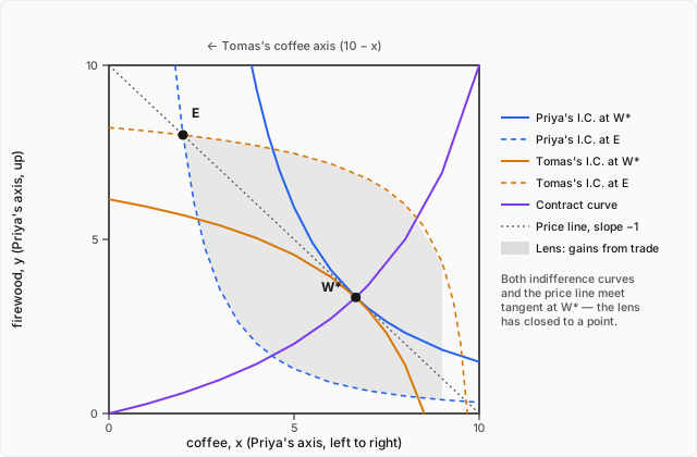
Because the two people's axes point opposite ways, their indifference curves open the opposite way too. Priya's preferences increase toward her own origin's far corner — up and to the right, more of both goods, exactly as always. Plotted on the same box, a curve that bows toward Priya's bottom-left origin (the standard convex shape from consumer-choice) is what her indifference curves look like. Tomas's preferences increase toward his origin, the top-right corner — so on this same page, his indifference curves bow the other way, toward the top-right. Two families of curves, same square, opening toward diagonally opposite corners: that is the picture, and everything else in this topic is read off it.

Why an off-curve point cannot be an equilibrium

Pick any allocation in the interior of the box where $MRS^P \neq MRS^T$ — say $MRS^P > MRS^T$. Recall what $MRS$ means, derived carefully in the consumer-choice topic: it is the rate, in units of $y$, at which a person is willing to trade $x$ away and feel no better or worse off. $MRS^P > MRS^T$ says Priya is willing to give up more firewood for one more sack of coffee than Tomas needs to receive to give one up. That gap is exploitable.

Suppose Priya gives Tomas $\Delta y$ units of firewood in exchange for $\Delta x$ units of coffee, at some rate $r = \Delta y / \Delta x$ chosen strictly between $MRS^T$ and $MRS^P$. Priya's utility changes, to first order, by

since $r < MRS^P$ by construction: Priya is paying less firewood per coffee than her own indifference curve says she'd accept. Tomas, giving up $\Delta x$ coffee and receiving $\Delta y = r\,\Delta x$ firewood, gains

since $r > MRS^T$: Tomas is receiving more firewood per coffee given up than his own indifference curve requires. Any rate $r$ strictly between the two $MRS$ values makes both people strictly better off. That whole range of mutually improving trades, swept out as $r$ varies across the gap, is a wedge-shaped region on the Edgeworth box bounded by the two people's indifference curves through the starting point — a lens. Wherever a lens exists, the starting allocation cannot be where trading stops, because both parties have something to gain by moving into it.

The lens closes exactly when the gap it depends on closes — when $MRS^P = MRS^T$. At that point the two indifference curves are tangent rather than crossing, there is no rate $r$ satisfying $MRS^T < r < MRS^P$ because the interval has shrunk to a single point, and no further mutually improving trade exists. This is the condition that will reappear, unchanged, three more times in this topic: as the definition of the contract curve, as the outcome of a competitive equilibrium, and as the content of the First Welfare Theorem. It is worth having derived it once, honestly, from nothing but the two people's own first-order conditions.

The contract curve

The locus of every allocation where the lens has closed — $MRS^P = MRS^T$ — is called the contract curve. Derive it in general before plugging in numbers. Write $\alpha_P = 2/3$ for Priya's coffee weight and $\alpha_T = 1/3$ for Tomas's, so from the Cobb-Douglas $MRS$ formula proven in consumer-choice, $MRS^i = \frac{\alpha_i}{1-\alpha_i}\cdot\frac{y_i}{x_i}$. Write $r_P = \frac{\alpha_P}{1-\alpha_P} = 2$ and $r_T = \frac{\alpha_T}{1-\alpha_T} = \frac12$. The tangency condition, with $x_T = 10 - x_P$ and $y_T = 10 - y_P$ substituted in, is

Plug in $r_P = 2$, $r_T = \tfrac12$:

Expand and collect the $y_P$ terms:

This is the contract curve for the Priya-Tomas economy — not one point, an entire curve of Pareto-efficient allocations, one for every $x_P$ between 0 and 10. Tabulate a few values:

It runs from $(0,0)$ — Priya's own origin, where she has nothing and Tomas has everything — to $(10,10)$ — Tomas's origin, the mirror-image extreme — sagging below the box's diagonal in between, because Priya's stronger taste for coffee ($\alpha_P > \alpha_T$) means an efficient split gives her a disproportionate share of coffee relative to firewood at every point along the curve. Every allocation on this curve satisfies $MRS^P = MRS^T$ by construction, so none of them has a lens; every allocation off it does.

Pareto efficiency, precisely — and its honest limit

Formally: an allocation is Pareto efficient if there is no other feasible allocation that makes at least one person strictly better off without making anyone else worse off. The argument just given proves the contract curve is exactly the set of Pareto-efficient allocations in this economy: off the curve, the lens supplies a Pareto improvement by construction; on the curve, $MRS^P = MRS^T$ removes every first-order direction of joint improvement, and convexity of both people's preferences (the same assumption that turned a stationary point into a genuine maximum for a single consumer in the consumer-choice topic) rules out a second-order escape as well.

Now say plainly what this buys and what it does not. Look again at the curve's own endpoints: $(0,0)$, where Priya has nothing at all and Tomas holds the entire $\bar X = 10, \bar Y = 10$. Is that Pareto efficient? Check the definition directly — is there a feasible reallocation that helps Priya without hurting Tomas? Any unit given to Priya has to come from Tomas's stock, and since Tomas's preferences are monotonic (more is better, from consumer-choice's four assumptions), removing anything from him makes him strictly worse off. So yes: Priya starving while Tomas has everything is Pareto efficient. Nothing about the definition objects to this in the slightest, because Pareto efficiency was never a statement about fairness — it is a statement about whether any value is being left unclaimed on the table, full stop. An allocation can waste nothing and still be a moral catastrophe; the two questions are simply different questions, and the theorems ahead answer only the first one. Keep that distinction in view for the rest of this topic, because it is exactly the distinction the Second Welfare Theorem is going to lean on.

Walrasian equilibrium: prices that clear every market at once

The contract curve says which allocations are efficient. It says nothing about which one, if any, decentralized trading among self-interested people actually reaches. That is a different question, and it needs a different piece of machinery: prices.

A Walrasian equilibrium (after Léon Walras) is a price ratio $p = p_x/p_y$ together with an allocation such that:

1. Each person, taking $p$ as given, chooses the utility-maximizing bundle subject to a budget constraint — but here is the one genuine novelty relative to consumer-choice's setup: there is no exogenous income $m$. Each person's wealth is simply the market value of what they walked in with:

Think of it as everyone selling their entire endowment at the going prices, then buying back whatever bundle they actually want — a bookkeeping fiction, but an exact one, since the constraint it produces, $p\,x_i + y_i = p\,e_x^i + e_y^i$, is precisely "the value of what you take home cannot exceed the value of what you brought." 2. Every market clears: $x_P + x_T = \bar X$ and $y_P + y_T = \bar Y$.

Solve it completely for Priya and Tomas. Normalize $p_y = 1$ so $p \equiv p_x$ is coffee's price in units of firewood. From the Cobb-Douglas demand formula proven in consumer-choice, $x_i^* = \alpha_i\, m_i/p$ and $y_i^* = (1-\alpha_i)\,m_i$. With $\alpha_P = \tfrac23$, $\alpha_T = \tfrac13$, $e^P=(2,8)$, $e^T=(8,2)$:

Impose market clearing in coffee, $x_P^* + x_T^* = 10$:

Multiply through by $3p$:

Coffee and firewood trade one-for-one. Now recover the full allocation. At $p=1$, $m_P = 2(1)+8=10$ and $m_T = 8(1)+2=10$ — by the coincidence of these particular numbers, the two endowments happen to have identical market value, ten dollars' worth each, even though they are made of completely different stuff.

Check market clearing directly. Coffee: $\tfrac{20}{3}+\tfrac{10}{3} = 10$. ✓ Firewood: $\tfrac{10}{3}+\tfrac{20}{3}=10$. ✓ Both markets clear exactly.

Check that this is the tangency the whole topic has been building toward. $MRS^P$ at $(\tfrac{20}{3},\tfrac{10}{3})$: $r_P\cdot y_P/x_P = 2\cdot\frac{10/3}{20/3} = 2\cdot\tfrac12 = 1$. $MRS^T$ at $(\tfrac{10}{3},\tfrac{20}{3})$: $r_T\cdot y_T/x_T = \tfrac12\cdot\frac{20/3}{10/3} = \tfrac12\cdot 2 = 1$. Both equal $1 = p$. ✓ And plug $x_P = \tfrac{20}{3}$ into the contract curve formula as a third, independent check: $y_P = \frac{10(20/3)}{40-3(20/3)} = \frac{200/3}{40-20} = \frac{200/3}{20} = \frac{10}{3}$. ✓ Exactly the equilibrium $y_P$. Three routes — clearing, tangency, and the contract-curve formula derived independently earlier — agree on the nose.

The trade itself makes the story concrete: Priya, who came in coffee-poor and firewood-rich, sells $8 - \tfrac{20}{3} = \tfrac43$ bundles of firewood and buys $\tfrac{20}{3}-2 = \tfrac{14}{3}$... — check the budget instead of eyeballing it: Priya sells firewood down from 8 to $\tfrac{10}{3}$, a reduction of $\tfrac{14}{3}$, and buys coffee up from 2 to $\tfrac{20}{3}$, a gain of $\tfrac{14}{3}$. At a one-for-one price this balances exactly, as it must. Both people's utility rises from $U(e) = 2^{2/3}\cdot8^{1/3} = 2^{5/3}\approx 3.17$ at the endowment to $U^*=\left(\tfrac{20}{3}\right)^{2/3}\left(\tfrac{10}{3}\right)^{1/3}\approx 5.29$ at equilibrium — the same number for both, again a coincidence of these particular symmetric numbers, not a general law.

Walras's law: why one market's clearing was actually enough

Notice something in the check above: once coffee cleared, firewood cleared too, without a second equation ever being solved. That is not a coincidence of these numbers — it is a theorem, and it is short enough to prove in full. Each person's budget constraint is an equality (monotonic preferences mean nobody leaves money on the table, exactly as in consumer-choice):

Sum this identity over both people. The left side becomes

using $e_x^P+e_x^T = \bar X$ and $e_y^P+e_y^T=\bar Y$ by definition of the total endowment. This sum is identically zero at every price, not just at equilibrium — it follows from nothing but each person's budget constraint holding with equality, which is true whether or not markets clear. Call the bracketed terms excess demand: $Z_x(p) \equiv (x_P+x_T)-\bar X$ and $Z_y(p) \equiv (y_P+y_T)-\bar Y$. Walras's law says

With two goods this has an immediate and useful consequence: if $Z_x(p)=0$ at some price, then $Z_y(p)=0$ automatically, since $p>0$. That is exactly what happened above — solving one clearing condition solved both, and it was never luck. With $n$ goods the same logic shows that only $n-1$ of the $n$ market-clearing conditions are independent, which is why a general-equilibrium price system pins down relative prices only, never an absolute price level — consistent with the homogeneity-of-degree-zero property already proven for individual demand in consumer-choice, now shown to survive aggregation across an entire economy.

The First Welfare Theorem

Here is the theorem Consumer Surplus, Producer Surplus, and Market Efficiency asserted but never proved: every Walrasian equilibrium is Pareto efficient. In this setting the proof is three lines, and every line of it has already been derived somewhere in this track.

Each person's own utility-maximization problem — proved in full in consumer-choice — sets their $MRS$ equal to the price ratio they face:

This is not two separate facts; it is the same number on the right of both equations, because a defining feature of a competitive market is that everybody faces the same price — nobody negotiates a private exchange rate, nobody knows or cares what the other person's preferences are. Priya solves her own optimization problem using only her own preferences and the two numbers $p_x, p_y$ posted for everyone. Tomas does the same, independently, using the identical two numbers. Since both equal the same $p_x/p_y$,

falls out immediately — and that is precisely the contract-curve condition derived earlier. A Walrasian equilibrium is a point on the contract curve. The numbers confirm it: $MRS^P=MRS^T=1$ at $\left(\tfrac{20}{3},\tfrac{10}{3}\right)$, already checked three ways above.

Sit with how little went into this. Nobody designed the outcome. Priya did not know Tomas's utility function; Tomas did not know Priya's. No planner compared their preferences and computed an efficient split — that computation, done explicitly in the contract-curve section, required knowing both people's exponents at once, information neither trader possessed or needed. Each of them solved a private optimization problem using nothing but their own preferences and a public price, and the coincidence of both problems using the same price is what forces their two private conditions to agree. That is the entire content of Adam Smith's invisible hand, stated as an actual theorem instead of a metaphor: decentralized self-interest, coordinated by nothing but a common price, reaches the same destination — no unclaimed gains from trade left anywhere — that would otherwise require a planner with more information than any single participant has.

The Second Welfare Theorem

The first theorem runs from prices to efficiency: start a competitive market anywhere, and it lands somewhere on the contract curve. The second theorem runs the argument in reverse: any point on the contract curve can be reached as a competitive equilibrium, provided endowments are redistributed first. Efficiency alone never picks out which point on the curve; this theorem says that picking one — on whatever grounds, fairness or politics or convention — does not require abandoning markets to get there. It requires only choosing the right starting endowments and then letting people trade.

State it precisely. Under convexity of preferences (the same assumption, once again, that made the single-consumer optimum a genuine maximum rather than a saddle), every Pareto-efficient allocation has, at that allocation, a common tangent line to both people's indifference curves — a price ratio that supports it. Redistribute the initial endowments to any point lying on that tangent line, and ordinary competitive trading, with no further intervention, converges on exactly that Pareto-efficient allocation.

Make it concrete with a point on the contract curve other than the one the original endowment happened to reach. Take $x_P = 5$: the contract-curve formula gives $y_P = \frac{10(5)}{40-15} = \frac{50}{25} = 2$, so this efficient allocation gives Priya $(5,2)$ and Tomas the rest, $(5,8)$. The supporting price ratio is the common $MRS$ there:

Both equal $p' = 0.8$, confirming this point is on the contract curve, exactly as the formula guarantees. Now find an endowment that makes $(5,2)/(5,8)$ the actual competitive equilibrium at this price. Any endowment on the line through $(5,2)$ with slope $-0.8$ works, because that line is precisely the set of bundles worth the same, at price $0.8$, as the target allocation. Take Priya's redistributed endowment to be $e_P' = (0, 6)$ — she now arrives with no coffee at all, six bundles of firewood — leaving Tomas $e_T' = (10, 4)$. Check the value: $0.8(0) + 6 = 6$ for Priya, and her demand at this wealth is $x_P^* = \tfrac23\cdot\frac{6}{0.8} = \tfrac23(7.5)=5$ and $y_P^*=\tfrac13(6)=2$ — exactly the target. ✓ For Tomas: $m_T' = 0.8(10)+4=12$, giving $x_T^*=\tfrac13\cdot\frac{12}{0.8}=\tfrac13(15)=5$ and $y_T^*=\tfrac23(12)=8$ — exactly his target too. ✓ Real trade happens along the way — Priya, starting with zero coffee, sells 4 bundles of firewood and buys 5 sacks of coffee, and at a price of $0.8$ that trade balances exactly ($4$ firewood sold $= 3.2$ coffee's worth $\div 0.8$... check directly: she spends $0.8\times 5 = 4$ on coffee, funded by selling $6-2=4$ firewood at a price of $1$ each — $4=4$. ✓). A hand redistributed the starting point; the market did everything after that.

Two honest caveats belong right next to the theorem, not in a footnote. First, convexity is doing real work: with non-convex preferences (or, once production is added back in, non-convex technology such as increasing returns to scale), some Pareto-efficient allocations have no supporting price at all — no common tangent exists, because the indifference curves bulge the wrong way at the point in question — so the theorem's guarantee simply fails for those allocations, no matter how endowments are shuffled. Second, and more practically: the redistribution above was a lump-sum transfer — endowments moved before anyone traded, with the transfer itself untouched by anything anyone did afterward. Genuinely lump-sum transfers are close to a theoretical fiction. A real government redistributing income does so through income taxes, sales taxes, or transfers keyed to earnings or purchases — and the moment a transfer depends on behavior, it stops being lump-sum and starts changing the relative price of doing the taxed thing, which is exactly the deadweight-loss mechanism proven in The Costs of Taxation: Deadweight Loss. The Second Welfare Theorem is a genuine result, not a debating trick — but it describes an idealized redistribution tool that essentially does not exist, which is precisely why real-world redistribution is not a free lunch even when the target allocation itself would be perfectly efficient.

What the theorems assume — and where every assumption has already broken

Put the two theorems together and they say something narrower and more useful than "markets are good": given price-taking behavior, no externalities, no public goods, complete markets, and full information, competitive equilibrium is Pareto efficient — and convexity is what lets any efficient outcome be reached by redistributing endowments rather than abandoning markets. That is a conditional, not a verdict, and this track has already spent several topics on exactly what happens when each condition fails.

Price-taking. The proof of the First Welfare Theorem used $MRS^P = p_x/p_y = MRS^T$, and that middle equality was doing the entire job — it exists only because both people treat $p$ as a fact of nature rather than a lever. A seller who instead sets price by restricting quantity — the subject of Monopoly — equates marginal revenue to marginal cost, not price to marginal cost, and that wedge is precisely a departure from the condition this proof needs. A market with a handful of large players negotiating strategically, as in Game Theory and Oligopoly, breaks the same assumption from a different direction.

No externalities. The proof assumed each person's optimization uses the true, complete cost or benefit of their own choice. Externalities and the Divergence of Private and Social Cost is a direct demonstration that this can fail even when every trade is fully voluntary and every price-taking condition holds perfectly — the tannery's private cost calculation was correct by its own lights and still wrong for society, because it never included the fishing co-op's bill. The First Welfare Theorem is silent about anything a transaction does to a bystander.

No public goods. The whole argument here assumed every good is rival and excludable — one more sack of coffee for Priya is genuinely one less for Tomas, which is what let a single point in the box represent a complete, mutually exclusive allocation. Public Goods and Common Resources covers goods where that is false, and an ordinary market has no mechanism to price them at all — there is no analogue of the Edgeworth box's feasibility constraint when consuming a good does not use it up.

Complete markets and full information. Every trade in this topic happened with both parties knowing exactly what was being exchanged and for what. Real economies are missing markets for enormous classes of future contingencies and carry pervasive information asymmetries between buyer and seller — neither has been touched by this track at all, and both are exactly the kind of gap that turns "efficient in principle" into "not efficient in this actual market."

None of this is a takedown of the theorems — they are correct, proven above from first principles, and remarkable on their own terms. It is the opposite move: naming precisely, rather than vaguely, the conditions a real market has to meet before the proof's conclusion is entitled to travel with it. Every deviation catalogued above is a topic this track has already built the tools to analyze quantitatively, which is the real payoff of doing the theorems last rather than first.

Worked example

Where this leads

Start from nothing but two people, two goods, and a fixed pie, and the whole apparatus of this track's earlier topics reassembles into something larger. The tangency condition from consumer-choice, applied independently by two people facing one shared price, becomes the First Welfare Theorem. The efficiency claim asserted without proof in the surplus topic gets its proof, and gets it with a precise scope attached — a scope this course has spent an entire sequence mapping the edges of, one broken assumption at a time: monopoly breaks price-taking, externalities break the private-cost calculation, public goods break excludability, and every one of those breakdowns already has its own topic and its own quantitative fix, because "the theorem doesn't apply here" was never a reason to stop measuring — it was the reason Externalities and Public Goods and Common Resources exist at all. This is the payoff of covering general equilibrium last: every exception in this closing section is a page you have already read, not a hand-wave.

That makes this a genuine capstone for the sequence that opened with Opportunity Cost and the Production Possibilities Frontier and Comparative Advantage — both of which quietly assumed a mechanism would exist for turning "everyone specializing" into "everyone actually trading." That mechanism, made completely explicit, is the Walrasian equilibrium built here.

But naming the assumptions honestly means naming what they leave standing outside this entire course, not just what has already been covered inside it. Three gaps in particular were never so much as touched. Every choice in every topic so far has been made under certainty — nobody has faced a genuine gamble, a bet on an unknown outcome, and the entire mathematics of risk is absent. Every trade has assumed both sides know exactly what they are buying and selling — nobody has hidden a used car's faults or a worker's true productivity, and asymmetric information is untouched. And every consumer has been a flawless constrained optimizer, with never a hint of the systematic ways real people's choices depart from that ideal — behavioral economics has not made an appearance. Each of those is not a footnote to microeconomics; each is close to a field of its own, and each is where this story picks back up.