Complex Analysis: Contour Integration and the Residue Theorem

Try to evaluate

\int_{-\infty}^{\infty}\frac{\cos x}{1+x^2}\,dx

using only the tools of ordinary calculus. Integration by parts pushes the derivative back and forth between $\cos x$ and $1/(1+x^2)$ without ever terminating. Substitution finds nothing to substitute. There is no elementary function whose derivative is $\cos x/(1+x^2)$ — not a gap in your technique, but a theorem: the antiderivative genuinely cannot be written using any finite combination of polynomials, exponentials, logarithms, and trigonometric functions. And yet the integral converges to a perfectly ordinary-looking number. It is $\pi/e$ .

Here is the strange part. That number falls out in about four lines, once you are willing to let $x$ — which has been a real number this entire time, on every page of this site so far — wander off the real line and roam through the complex plane instead. You compute one residue, a single number extracted from a single point, multiply it by $2\pi i$ , and the answer is sitting in front of you. This is not a trick restricted to this one integral; it is a general method, and by the end of this topic you will run it in full on a simpler cousin of the integral above, then come back and cash in on this one. To get there we need four ideas: what it means for a complex function to be well-behaved, a theorem about integrating such functions around closed loops, the concept of a residue, and the theorem that ties a residue to the value of an integral.

Analytic functions and the Cauchy-Riemann equations

A complex function $f$ assigns a complex number to a complex number, $f(z)=f(x+iy)$ . Split it into real and imaginary parts,

f(z) = u(x,y) + iv(x,y),

where $u$ and $v$ are ordinary real-valued functions of the two real variables $x,y$ . Nothing so far is more than bookkeeping — every complex function is secretly a pair of real functions of two real variables.

The interesting question is whether $f$ has a derivative. Define it exactly as in ordinary calculus,

f'(z) = \lim_{h\to0}\frac{f(z+h)-f(z)}{h},

but now notice something that never came up for real functions: $h$ is a complex number, so it can approach $0$ from any direction in the plane — along the real axis, along the imaginary axis, spiraling in, anything. A real function only ever had two directions to worry about, left and right, and they had to agree. A complex function has infinitely many directions, and for the limit to exist, all of them must agree on the same value. This is an enormously more restrictive demand, and functions that satisfy it are called analytic (or holomorphic) at that point.

To see what the demand costs, evaluate the limit along two particular directions and require them to match. Along the real axis, $h$ is a small real number, and

f'(z) = \lim_{h\to0}\frac{f(x+h,y)-f(x,y)}{h} = \frac{\partial u}{\partial x} + i\frac{\partial v}{\partial x}.

Along the imaginary axis, $h=ik$ for small real $k$ , and

f'(z) = \lim_{k\to0}\frac{f(x,y+k)-f(x,y)}{ik} = \frac{1}{i}\left(\frac{\partial u}{\partial y}+i\frac{\partial v}{\partial y}\right) = \frac{\partial v}{\partial y} - i\frac{\partial u}{\partial y}.

These two expressions for $f'(z)$ must be the identical complex number. Matching real parts and matching imaginary parts gives the Cauchy-Riemann equations:

\frac{\partial u}{\partial x} = \frac{\partial v}{\partial y}, \qquad \frac{\partial u}{\partial y} = -\frac{\partial v}{\partial x}.

A function is analytic on a region exactly when $u$ and $v$ have continuous partial derivatives there satisfying these two equations at every point. Polynomials in $z$ , $e^z$ , $\sin z$ , $\cos z$ , and $1/z$ (away from $z=0$ ) are all analytic wherever they are defined; a function as simple-looking as $f(z)=\bar z=x-iy$ is not analytic anywhere, since here $u=x,v=-y$ gives $\partial u/\partial x=1$ but $\partial v/\partial y=-1$ , and the equations fail at every point. Analyticity is a genuine, checkable restriction, not a technicality.

Cauchy's integral theorem

Everything that follows rests on one theorem about integrating an analytic function around a closed loop. Let $C$ be a simple closed curve (one that does not cross itself) traversed counterclockwise, and suppose $f$ is analytic everywhere on $C$ and everywhere inside it. Then

\oint_C f(z)\,dz = 0.

This is Cauchy's integral theorem, and it is not an assumption — it follows directly from the Cauchy-Riemann equations, by a route that should look familiar. Write $dz=dx+i\,dy$ and expand:

f(z)\,dz = (u+iv)(dx+i\,dy) = (u\,dx - v\,dy) + i(v\,dx+u\,dy).

Each of the two bracketed expressions is a real line integral of the form $\oint(P\,dx+Q\,dy)$ , and Green's theorem converts each into an area integral:

\oint_C (P\,dx+Q\,dy) = \iint_D \left(\frac{\partial Q}{\partial x}-\frac{\partial P}{\partial y}\right)dA.

For the real part, $P=u,\ Q=-v$ , so the integrand becomes $-\partial v/\partial x - \partial u/\partial y$ . The Cauchy-Riemann equations say $\partial u/\partial y=-\partial v/\partial x$ , so this is $-\partial v/\partial x-(-\partial v/\partial x)=0$ . For the imaginary part, $P=v,\ Q=u$ , and the integrand becomes $\partial u/\partial x-\partial v/\partial y$ , which the other Cauchy-Riemann equation sets to zero directly. Both area integrals vanish identically, so the loop integral vanishes:

\oint_C f(z)\,dz = 0.

This is exactly the fact already met as curl-free fields: a vector field integrates to zero around every closed loop precisely when its curl vanishes. Cauchy's theorem is that same statement, applied simultaneously to the two real vector fields $(u,-v)$ and $(v,u)$ built from an analytic function's real and imaginary parts — and the Cauchy-Riemann equations are exactly what force both curls to vanish at once. Analyticity is curl-freeness, worn as a disguise.

Cauchy's integral formula

Cauchy's theorem has a companion that turns out to be even more useful. Suppose $f$ is analytic on and inside a closed contour $C$ , and $a$ is some point strictly inside $C$ . Then

f(a) = \frac{1}{2\pi i}\oint_C \frac{f(z)}{z-a}\,dz.

This says something remarkable: the value of an analytic function anywhere inside a loop is completely determined by its values on the loop. To see why, notice that $f(z)/(z-a)$ is analytic everywhere inside $C$ except at the single point $z=a$ . Shrink the original contour down to a tiny circle of radius $\epsilon$ centered at $a$ ; Cauchy's theorem, applied to the ring-shaped region between the two contours (where the integrand is analytic throughout), guarantees the two contour integrals are equal. So

\oint_C \frac{f(z)}{z-a}\,dz = \oint_{|z-a|=\epsilon} \frac{f(z)}{z-a}\,dz.

Parametrize the small circle as $z=a+\epsilon e^{i\theta}$ , so $dz=i\epsilon e^{i\theta}\,d\theta$ and $z-a=\epsilon e^{i\theta}$ :

\oint_{|z-a|=\epsilon}\frac{f(z)}{z-a}\,dz = \int_0^{2\pi}\frac{f(a+\epsilon e^{i\theta})}{\epsilon e^{i\theta}}\,i\epsilon e^{i\theta}\,d\theta = i\int_0^{2\pi}f(a+\epsilon e^{i\theta})\,d\theta.

The radius $\epsilon$ has canceled completely out of the integrand. Now let $\epsilon\to0$ : since $f$ is continuous, $f(a+\epsilon e^{i\theta})\to f(a)$ for every $\theta$ , and the integral becomes

i\int_0^{2\pi}f(a)\,d\theta = 2\pi i\,f(a).

Putting the two results together gives Cauchy's integral formula. Differentiating both sides with respect to $a$ , $n$ times, under the integral sign — a mechanical but slightly lengthy step, not repeated here — produces the generalized version for derivatives:

f^{(n)}(a) = \frac{n!}{2\pi i}\oint_C \frac{f(z)}{(z-a)^{n+1}}\,dz.

This single formula, turning an $n$ th derivative into a contour integral, is going to reappear by name in the closing section of this topic.

Poles and residues

Suppose $f$ fails to be analytic at an isolated point $a$ , but is analytic everywhere in a small punctured disk around it. If $(z-a)^nf(z)$ stays finite and nonzero as $z\to a$ for some positive integer $n$ , then $a$ is called a pole of order $n$ . Near such a point, $f$ has a Laurent series — an ordinary power series extended to include a finite number of negative powers of $(z-a)$ :

f(z) = \frac{c_{-n}}{(z-a)^n}+\cdots+\frac{c_{-1}}{z-a}+c_0+c_1(z-a)+\cdots

Every coefficient here carries information about $f$ , but one of them is special: the coefficient of $1/(z-a)$ , called the residue of $f$ at $a$ and written $\operatorname{Res}_{z=a}f$ .

Here is why it is special. Integrate the Laurent series term by term around a tiny circle centered at $a$ . Parametrizing as before, $z=a+\epsilon e^{i\theta}$ ,

\oint_{|z-a|=\epsilon}(z-a)^k\,dz = \int_0^{2\pi}\epsilon^ke^{ik\theta}\,i\epsilon e^{i\theta}\,d\theta = i\epsilon^{k+1}\int_0^{2\pi}e^{i(k+1)\theta}\,d\theta,

for any integer $k$ (positive, negative, or zero). If $k\neq-1$ , the exponent $k+1$ is a nonzero integer, and $\int_0^{2\pi}e^{i(k+1)\theta}\,d\theta=0$ , since a nonzero-frequency complex exponential integrates to zero over a full period. But if $k=-1$ , the exponential disappears entirely: $\int_0^{2\pi}1\,d\theta=2\pi$ , and the prefactor $\epsilon^{k+1}=\epsilon^0=1$ is independent of $\epsilon$ . So every term in the Laurent series integrates to zero except the $1/(z-a)$ term, which contributes exactly $2\pi i\,c_{-1}$ . That is,

\oint_{|z-a|=\epsilon}f(z)\,dz = 2\pi i\operatorname{Res}_{z=a}f.

Out of an entire infinite series of coefficients, integration is a filter that lets exactly one of them through. For a simple pole ( $n=1$ ), the residue has a convenient shortcut:

\operatorname{Res}_{z=a}f = \lim_{z\to a}(z-a)f(z).

In particular, for a ratio $f(z)=p(z)/q(z)$ where $q$ has a simple zero at $a$ (so $q(a)=0$ but $q'(a)\neq0$ ), L'Hôpital's rule applied to this limit gives the frequently useful form

\operatorname{Res}_{z=a}f = \frac{p(a)}{q'(a)}.

The residue theorem

Now combine everything. Suppose $f$ is analytic on and inside a closed contour $C$ , except for finitely many isolated poles $a_1,\ldots,a_N$ located strictly inside $C$ . Cut a tiny circle out around each pole and connect each one to $C$ with a thin corridor; on the resulting region, with all the poles excised, $f$ is analytic everywhere, so Cauchy's theorem applies and the integral around the whole boundary of this region is zero. The corridor contributions are traversed once in each direction and cancel exactly. What remains is $C$ itself, traversed counterclockwise, together with the small circles around each pole, traversed clockwise (since they are cut out of the region). Flipping their orientation back to counterclockwise introduces a sign, giving the residue theorem:

\oint_C f(z)\,dz = 2\pi i\sum_{k=1}^N \operatorname{Res}_{z=a_k}f.

An entire loop integral, however complicated the function looks elsewhere in the plane, collapses to a finite sum of numbers extracted at isolated points.

Closing the contour: turning a real integral into a complex one

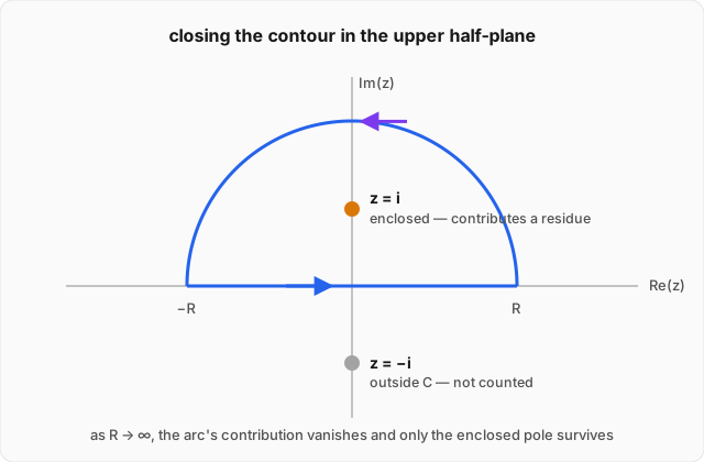
The residue theorem is a statement about closed loops in the complex plane, but the integral we started with runs along the entire real line. The bridge between them is a standard construction called closing the contour. Build a closed loop $C_R$ out of two pieces: the straight segment from $-R$ to $R$ along the real axis, and a semicircular arc $\Gamma_R$ of radius $R$ in the upper half-plane connecting $R$ back to $-R$ . As $R\to\infty$ , the straight piece becomes the entire real-line integral we want.

Everything hinges on what happens to the arc. If $|f(z)|$ falls off fast enough as $|z|\to\infty$ in the upper half-plane, the arc's contribution vanishes in the limit, by the estimation lemma: if $|f(z)|\leq M_R$ everywhere on $\Gamma_R$ , then

\left|\int_{\Gamma_R}f(z)\,dz\right| \leq M_R\cdot(\text{length of }\Gamma_R) = M_R\cdot\pi R.

For a ratio of polynomials whose denominator degree exceeds the numerator degree by two or more, $M_R\sim1/R^2$ , and $M_R\cdot\pi R\to0$ . For integrands carrying an oscillating factor $e^{iz}$ instead — which only decays in the upper half-plane, since for $z=x+iy$ with $y>0$ , $|e^{iz}|=|e^{ix}e^{-y}|=e^{-y}<1$ — a sharper argument called Jordan's lemma shows the arc still vanishes even when the remaining factor only decays as slowly as $1/R$ . Either way, once the arc is shown to vanish,

\int_{-\infty}^{\infty}f(x)\,dx = \lim_{R\to\infty}\oint_{C_R}f(z)\,dz = 2\pi i\sum(\text{residues enclosed in the upper half-plane}).

A real integral over an infinite line has become a finite sum of residues, provided you can show the far-away arc contributes nothing.

Closing the contour: the real line from minus R to R, plus a semicircular arc through the upper half-plane, encloses only the poles above the real axis — here the one at z equals positive i, but not the one at minus i.

Worked example

Evaluate $\displaystyle\int_{-\infty}^{\infty}\frac{dx}{1+x^2}$ by contour integration, showing every step: closing the contour, identifying the enclosed pole, computing the residue, and applying the residue theorem. (click to reveal the solution)

Setting up: extend the integrand to the complex plane, $f(z)=\dfrac{1}{1+z^2}$ . Factor the denominator:

1+z^2 = (z-i)(z+i),

so $f$ has two simple poles, at $z=i$ and $z=-i$ , and is analytic everywhere else.

Closing the contour: build $C_R$ from the real segment $[-R,R]$ together with the semicircular arc $\Gamma_R:\ z=Re^{i\theta},\ \theta\in[0,\pi]$ , closing the loop in the upper half-plane.

Showing the arc vanishes: on $\Gamma_R$ , the reverse triangle inequality gives

|1+z^2| = |z^2-(-1)| \geq |z|^2-1 = R^2-1,

|f(z)| \leq \frac{1}{R^2-1} \quad\text{everywhere on }\Gamma_R.

The arc has length $\pi R$ , so by the estimation lemma,

\left|\int_{\Gamma_R}f(z)\,dz\right| \leq \frac{1}{R^2-1}\cdot\pi R = \frac{\pi R}{R^2-1}\xrightarrow[R\to\infty]{}0.

The arc contributes nothing in the limit.

Identifying the enclosed pole: the upper-half-plane contour $C_R$ , for any $R>1$ , encloses $z=i$ (since $|i|=1<R$ and $i$ lies above the real axis) but not $z=-i$ (which lies below the real axis, outside the region enclosed by this particular contour).

Computing the residue: since $z=i$ is a simple pole,

\operatorname{Res}_{z=i}f = \lim_{z\to i}(z-i)\cdot\frac{1}{(z-i)(z+i)} = \frac{1}{i+i} = \frac{1}{2i}.

Applying the residue theorem:

\oint_{C_R}f(z)\,dz = 2\pi i\cdot\frac{1}{2i} = \pi.

Taking the limit: the left side splits into the straight segment and the arc,

\oint_{C_R}f(z)\,dz = \int_{-R}^{R}\frac{dx}{1+x^2} + \int_{\Gamma_R}f(z)\,dz.

As $R\to\infty$ , the arc term vanishes and the segment term becomes the full real-line integral, so

\int_{-\infty}^{\infty}\frac{dx}{1+x^2} = \pi.

Checking the result: this integral also has an elementary antiderivative, $\arctan x$ , and

\int_{-\infty}^{\infty}\frac{dx}{1+x^2} = \Big[\arctan x\Big]_{-\infty}^{\infty} = \frac{\pi}{2}-\left(-\frac{\pi}{2}\right) = \pi,

exactly matching the contour-integration answer. This is reassuring precisely because it is a case where you could check the machinery against an answer obtained the ordinary way — before turning it loose, in the next section, on an integral that offers no such elementary check.

Cashing in the trick: the integral we started with

Return to $\displaystyle\int_{-\infty}^\infty\frac{\cos x}{1+x^2}\,dx$ , the integral with no elementary antiderivative. The move is to stop looking at $\cos x$ directly and instead consider

\int_{-\infty}^{\infty}\frac{e^{ix}}{1+x^2}\,dx.

Since $1+x^2$ is real and $e^{ix}=\cos x+i\sin x$ , this integral's real part is exactly $\int\cos x/(1+x^2)\,dx$ , and its imaginary part is $\int\sin x/(1+x^2)\,dx$ , which vanishes automatically because $\sin x/(1+x^2)$ is an odd function integrated over a symmetric interval. So computing the complex integral hands back the real one, for free, as its real part.

The function $g(z)=e^{iz}/(1+z^2)$ has the same two poles as before, at $z=\pm i$ , and the same contour closes it: on the upper-half-plane arc, $z=Re^{i\theta}$ with $\theta\in[0,\pi]$ , so $|e^{iz}|=e^{-R\sin\theta}\leq1$ , while $|1/(1+z^2)|\leq1/(R^2-1)$ as before. The same estimation-lemma bound applies without needing Jordan's lemma at all here — the polynomial factor alone already decays like $1/R^2$ , and $|e^{iz}|\leq1$ throughout the upper half-plane is enough to keep the product decaying just as fast, so the arc vanishes as $R\to\infty$ exactly as in the worked example.

Only $z=i$ is enclosed. The residue there is

\operatorname{Res}_{z=i}g = \lim_{z\to i}(z-i)\cdot\frac{e^{iz}}{(z-i)(z+i)} = \frac{e^{i(i)}}{2i} = \frac{e^{-1}}{2i}.

By the residue theorem,

\oint_{C_R}g(z)\,dz = 2\pi i\cdot\frac{e^{-1}}{2i} = \frac{\pi}{e}.

Taking $R\to\infty$ exactly as before,

\int_{-\infty}^{\infty}\frac{e^{ix}}{1+x^2}\,dx = \frac{\pi}{e}.

The right side is already a real number, consistent with the vanishing imaginary part noted above, and it is entirely the real part:

\int_{-\infty}^{\infty}\frac{\cos x}{1+x^2}\,dx = \frac{\pi}{e}.

The number promised at the very start of this topic drops out of exactly one residue calculation — the same pole, $z=i$ , doing the same job it did in the worked example, just carrying one extra factor of $e^{iz}$ along for the ride.

Where this leads

The residue theorem is not a curiosity confined to definite integrals. Real integrals that show up throughout physics as Fourier transforms of decaying or oscillating signals — exactly the kind built on Fourier analysis — are routinely evaluated this same way: extend the integrand to the complex plane, close the contour, read off the residues.

There is also a much closer connection, one flagged explicitly at the end of the special functions topic. Rodrigues' formula generates the Legendre polynomials as an $l$ -th derivative,

P_l(x) = \frac{1}{2^ll!}\frac{d^l}{dx^l}\left(x^2-1\right)^l.

Apply the generalized Cauchy integral formula from earlier in this topic, $f^{(n)}(a)=\dfrac{n!}{2\pi i}\displaystyle\oint_C\dfrac{f(z)}{(z-a)^{n+1}}\,dz$ , to $f(z)=(z^2-1)^l$ with $n=l$ and $a=x$ :

\frac{d^l}{dz^l}(z^2-1)^l\bigg|_{z=x} = \frac{l!}{2\pi i}\oint_C\frac{(t^2-1)^l}{(t-x)^{l+1}}\,dt.

Substituting this into Rodrigues' formula, the two factors of $l!$ cancel:

P_l(x) = \frac{1}{2^ll!}\cdot\frac{l!}{2\pi i}\oint_C\frac{(t^2-1)^l}{(t-x)^{l+1}}\,dt = \frac{1}{2\pi i}\oint_C\frac{(t^2-1)^l}{2^l(t-x)^{l+1}}\,dt.

This is Schläfli's integral representation of the Legendre polynomials — the same functions built by repeated differentiation on that earlier page, rebuilt here as a single contour integral, with the differentiation itself packaged inside the generalized Cauchy formula derived above. A derivative repeated $l$ times and a loop integral around one point turn out to be the same object, viewed from two different angles.