Special Functions: Legendre Polynomials and Spherical Harmonics

Every uniform sphere looks identical from every direction — but nothing real is a perfectly uniform sphere. A planet bulges very slightly at the equator. An atom's electron cloud is almost never a perfect ball; most of the interesting ones are lopsided in a specific, repeatable way. The moment a source of gravity, charge, or a quantum wave function departs even slightly from perfect spherical symmetry, its potential or its wave function outside picks up genuine angle dependence: it becomes a function of the polar angle $\theta$ and azimuthal angle $\phi$ , not of the radius $r$ alone. How do you organize that angular dependence into calculable pieces?

This is precisely the question the previous topic leaves as unfinished business. Separation of variables was used there on a string, in one spatial dimension with two endpoints. The natural next PDE, not yet solved anywhere on this site, is the three-dimensional version of Laplace's equation — the same equation quietly used inside Coulomb's law and behind the Schrödinger equation for any atom — written not on a line, but in the spherical geometry that atoms and planets actually have.

Laplace's equation in spherical coordinates

The Laplacian $\nabla^2\equiv\nabla\cdot\nabla$ is built from exactly the divergence and gradient operators constructed in vector calculus: apply the gradient to get a vector field, then take its divergence to get back a scalar. In spherical coordinates $(r,\theta,\phi)$ , working through that same chain rule (a lengthier but entirely mechanical calculation, not repeated here) gives the Laplacian of a scalar function $u(r,\theta,\phi)$ as

\nabla^2u=\frac{1}{r^2}\frac{\partial}{\partial r}\left(r^2\frac{\partial u}{\partial r}\right) +\frac{1}{r^2\sin\theta}\frac{\partial}{\partial\theta}\left(\sin\theta\frac{\partial u}{\partial\theta}\right) +\frac{1}{r^2\sin^2\theta}\frac{\partial^2u}{\partial\phi^2}.

Laplace's equation, $\nabla^2u=0$ , describes a potential in any region with no charge or mass — exactly the situation outside a lopsided planet or a nonspherical charge distribution. Now separate variables, exactly as in the previous topic, by assuming

u(r,\theta,\phi)=R(r)Y(\theta,\phi).

Separating radius from angle

Substituting the product form into $\nabla^2u=0$ and multiplying through by $r^2/[R(r)Y(\theta,\phi)]$ gives

\frac{1}{R}\frac{d}{dr}\left(r^2\frac{dR}{dr}\right) +\frac{1}{Y}\left[\frac{1}{\sin\theta}\frac{\partial}{\partial\theta}\left(\sin\theta\frac{\partial Y}{\partial\theta}\right)+\frac{1}{\sin^2\theta}\frac{\partial^2Y}{\partial\phi^2}\right]=0.

The first term depends only on $r$ ; the bracketed term, divided by $Y$ , depends only on the angles. By the same reasoning used for the vibrating string, both must equal a constant, with opposite signs so their sum is zero. Write that constant as $l(l+1)$ — a strange-looking choice for now, justified only once the angular equation is actually solved and single-valued, non-blowing-up solutions are demanded:

\frac{1}{R}\frac{d}{dr}\left(r^2\frac{dR}{dr}\right)=l(l+1),

\frac{1}{\sin\theta}\frac{\partial}{\partial\theta}\left(\sin\theta\frac{\partial Y}{\partial\theta}\right)+\frac{1}{\sin^2\theta}\frac{\partial^2Y}{\partial\phi^2}=-l(l+1)Y.

The radial equation is solved by a power law. Try $R(r)=r^n$ : then $r^2R'=nr^{n+1}$ , and $\frac{d}{dr}(nr^{n+1})=n(n+1)r^n$ , so the radial equation demands $n(n+1)=l(l+1)$ , whose two roots are $n=l$ and $n=-(l+1)$ . The general radial solution is therefore

R(r)=Ar^l+\frac{B}{r^{l+1}}.

The $r^l$ piece is the part of the potential that must vanish at the origin if there is no source there; the $1/r^{l+1}$ piece is the part that falls off with distance, generalizing the familiar $1/r$ potential of a point charge (which is exactly the $l=0$ case).

Separating the angular equation, and where the integer $m$ is born

The angular equation still mixes $\theta$ and $\phi$ . Separate again: $Y(\theta,\phi)=\Theta(\theta)\Phi(\phi)$ . Substituting and multiplying through by $\sin^2\theta/(\Theta\Phi)$ gives

\frac{\sin\theta}{\Theta}\frac{d}{d\theta}\left(\sin\theta\frac{d\Theta}{d\theta}\right)+l(l+1)\sin^2\theta=-\frac{\Phi''(\phi)}{\Phi(\phi)}.

The left side depends only on $\theta$ , the right only on $\phi$ , so both equal a new constant, called $m^2$ :

\Phi''(\phi)=-m^2\Phi(\phi).

This is, once again, the same equation solved on the ordinary differential equations page and used throughout Fourier analysis: purely imaginary characteristic roots $r=\pm im$ , giving $\Phi(\phi)=e^{im\phi}$ . But here a new physical requirement enters that a string or an infinite line never had: $\phi$ is an angle, and going around once, $\phi\to\phi+2\pi$ , must return you to the same point in space, so $\Phi$ must satisfy

e^{im(\phi+2\pi)}=e^{im\phi} \quad\Longrightarrow\quad e^{2\pi im}=1.

That forces $m$ to be an integer. This is exactly the integer $m$ already met on the page about angular momentum and spin, where it appeared as the eigenvalue label of $\hat L_z$ , produced there by a completely different argument — an algebraic ladder built from raising and lowering operators, with no reference to any differential equation at all. Here the same integer falls out of a geometric requirement: single-valuedness on a circle. Two derivations, built from entirely different tools, landing on the identical quantization. That is not a coincidence to shrug off; it is a sign that both derivations are describing the same underlying structure from different angles.

Legendre's equation and Legendre polynomials

What remains is the $\theta$ -equation, with $m$ now fixed:

\sin\theta\frac{d}{d\theta}\left(\sin\theta\frac{d\Theta}{d\theta}\right)+\left[l(l+1)\sin^2\theta-m^2\right]\Theta=0.

Substitute $x=\cos\theta$ , so $x$ runs over $[-1,1]$ as $\theta$ runs over $[0,\pi]$ , and $\frac{d}{d\theta}=-\sin\theta\,\frac{d}{dx}$ . Carrying this substitution through converts the equation into the associated Legendre equation,

\frac{d}{dx}\left[(1-x^2)\frac{d\Theta}{dx}\right]+\left[l(l+1)-\frac{m^2}{1-x^2}\right]\Theta=0.

The case $m=0$ — no dependence on the azimuthal angle at all, the axially symmetric case relevant to a charge distribution or planet that bulges only along one axis — reduces this to plain Legendre's equation:

\frac{d}{dx}\left[(1-x^2)\frac{dP}{dx}\right]+l(l+1)P=0.

For $l=0,1,2,\ldots$ , the solutions that stay finite at $x=\pm1$ (that is, at the poles $\theta=0,\pi$ , where a physically sensible potential cannot blow up) are polynomials of degree $l$ , the Legendre polynomials $P_l(x)$ , generated compactly by Rodrigues' formula:

P_l(x)=\frac{1}{2^ll!}\frac{d^l}{dx^l}\left(x^2-1\right)^l.

For $m\neq0$ , the solutions are the associated Legendre functions $P_l^m(x)$ , and reuniting the angular pieces gives the full angular solution, the spherical harmonics:

Y_l^m(\theta,\phi)=N_{lm}\,P_l^{\,m}(\cos\theta)\,e^{im\phi},

with $N_{lm}$ a normalization constant. Just as before, regularity of $P_l^m$ at the poles restricts $m$ to the integers $-l,-l+1,\ldots,l-1,l$ — precisely the range $m=-l,\ldots,l$ already stated, but never derived, on the angular-momentum-and-spin page. The spherical harmonics are simultaneous eigenfunctions of $\hat L^2$ and $\hat L_z$ ,

\hat L^2Y_l^m=\hbar^2l(l+1)Y_l^m, \qquad \hat L_zY_l^m=\hbar mY_l^m,

with exactly the eigenvalues that page assigned to the abstract states $|l,m\rangle$ . This is where those integer labels actually come from: not an assumption about how nature likes to count, but the requirement that an angular solution to Laplace's equation (or to the angular part of the Schrödinger equation, which separates the same way for any spherically symmetric potential $V(r)$ ) be single-valued and finite everywhere on the sphere, including its two awkward poles.

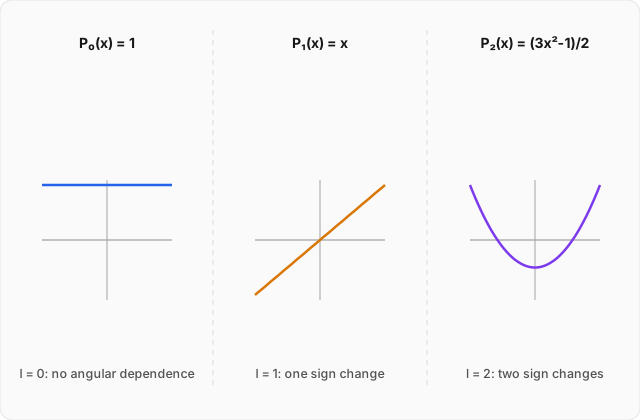
Three panels, each plotting one Legendre polynomial as a curve over the interval from x equals negative one to positive one: a flat horizontal line for P-zero, a straight diagonal line through the origin for P-one, and a symmetric upward-curving parabola-like shape for P-two. — The first three Legendre polynomials, each one degree higher than the last, generated by taking x squared minus one to the l-th power, differentiating it l times, and rescaling.

Worked example

Use Rodrigues' formula to derive $P_0(x)$ , $P_1(x)$ , and $P_2(x)$ , verify that $P_2$ satisfies Legendre's equation for $l=2$ , and check that $P_1$ and $P_2$ are orthogonal on $[-1,1]$ . (click to reveal the solution)

Deriving $P_0$ : with $l=0$ ,

P_0(x)=\frac{1}{2^0\,0!}\frac{d^0}{dx^0}(x^2-1)^0=1,

since $(x^2-1)^0=1$ and the "zeroth derivative" of a function is just the function itself. So $P_0(x)=1$ , a constant — consistent with the fact that the $l=0$ angular solution has no angular dependence at all, matching a plain, spherically symmetric $1/r$ potential.

Deriving $P_1$ : with $l=1$ ,

P_1(x)=\frac{1}{2^1\,1!}\frac{d}{dx}(x^2-1)=\frac{1}{2}(2x)=x.

Deriving $P_2$ : with $l=2$ ,

P_2(x)=\frac{1}{2^2\,2!}\frac{d^2}{dx^2}(x^2-1)^2=\frac{1}{8}\frac{d^2}{dx^2}\left(x^4-2x^2+1\right).

The first derivative of $x^4-2x^2+1$ is $4x^3-4x$ , and the second derivative is $12x^2-4$ . Therefore

P_2(x)=\frac{1}{8}\left(12x^2-4\right)=\frac{3x^2-1}{2}.

Verifying $P_2$ solves Legendre's equation for $l=2$ : the equation to check is

\frac{d}{dx}\left[(1-x^2)\frac{dP_2}{dx}\right]+6P_2=0

(using $l(l+1)=2\cdot3=6$ ). Compute each piece. First,

P_2'(x)=\frac{d}{dx}\left(\frac{3x^2-1}{2}\right)=3x.

Then

(1-x^2)P_2'(x)=(1-x^2)(3x)=3x-3x^3,

and differentiating again,

\frac{d}{dx}\left(3x-3x^3\right)=3-9x^2.

Adding the second term, $6P_2=6\cdot\frac{3x^2-1}{2}=9x^2-3$ :

\left(3-9x^2\right)+\left(9x^2-3\right)=0.

The equation is satisfied identically, for every $x$ , confirming $P_2(x)=\frac{3x^2-1}{2}$ is genuinely a solution of Legendre's equation with $l=2$ .

Checking orthogonality of $P_1$ and $P_2$ : Legendre polynomials of different degree are orthogonal on $[-1,1]$ under the plain integral inner product, the same structure used for sines and cosines in Fourier analysis. Directly:

\int_{-1}^{1}P_1(x)P_2(x)\,dx=\int_{-1}^{1}x\cdot\frac{3x^2-1}{2}\,dx=\int_{-1}^{1}\frac{3x^3-x}{2}\,dx.

The integrand $\frac{3x^3-x}{2}$ is an odd function of $x$ (built entirely from odd powers), and the integral of any odd function over a symmetric interval $[-1,1]$ vanishes:

\int_{-1}^{1}\frac{3x^3-x}{2}\,dx=0.

So $P_1$ and $P_2$ are indeed orthogonal — the same phenomenon seen for the trigonometric basis, now appearing for an entirely different family of functions, born from a completely different differential equation.

Where this leads

Legendre polynomials and spherical harmonics are the angular vocabulary for every problem in physics with a natural center: the electric potential of any real, imperfectly spherical charge distribution, the gravitational field of any real, imperfectly spherical planet, and above all the actual angular wave functions of the hydrogen atom, whose radial equation this page's $R(r)=Ar^l+B/r^{l+1}$ is the source-free special case of. The integer $l$ and $m$ found here by demanding regularity are precisely the orbital quantum numbers already used, but not derived, on the page about angular momentum and spin — two roads, algebraic and differential, arriving at the same integers. Rodrigues' formula itself has a further life ahead: it can be rewritten as a contour integral in the complex plane, a connection that becomes available once complex analysis and contour integration enters this track.