Vector Calculus: Line, Surface, and Volume Integrals

The previous topic built three tools for a single question: given a field, what is it doing right here, at this one point? But most of the physics we actually want to compute is global, not local — the total work done moving all the way along a path, the total flux passing through an entire surface, the total charge inside an entire volume. Differentiation zooms in; this topic is about zooming back out, and about the two remarkable theorems that connect the local picture to the global one without losing a single detail in between.

Line integrals: work, generalized

Work and energy defined work for motion along a straight line: $W = \int F\,dx$ . A force rarely acts along a straight line in general, and a path is rarely straight either. The line integral generalizes this fully:

W = \int_C \vec F \cdot d\vec l,

where $C$ is some path through space and $d\vec l$ is an infinitesimal displacement along that path, tangent to it at every point. The dot product does exactly the job you'd expect: it keeps only the component of $\vec F$ pointing along the direction of travel at each instant, exactly as $\cos\theta$ did in the original definition of work — this is that same idea, just no longer restricted to straight lines or constant forces.

Surface integrals: flux

A surface integral measures how much of a field passes through a surface — its flux:

\Phi = \int_S \vec F\cdot d\vec A,

where $d\vec A = \hat n\,dA$ is an infinitesimal patch of the surface, represented as a vector: its magnitude is the patch's area, and its direction is the outward-pointing normal to the surface at that patch. Picture $\vec F$ as the velocity field of a flowing fluid: $\vec F\cdot d\vec A$ at each patch measures how much fluid crosses that patch per unit time (fluid moving parallel to the surface, tangent to it, contributes nothing — only the component punching straight through counts), and the integral adds this up over the whole surface. A field pointing straight through a surface everywhere gives a large flux; a field that grazes the surface everywhere, staying tangent to it, gives zero.

Volume integrals

The most familiar generalization: integrate a scalar field $f$ over a three-dimensional region,

\int_V f\,dV,

adding up a small contribution $f\,dV$ from every infinitesimal piece of volume in the region. Nothing conceptually new here — it's the ordinary Riemann-sum idea from single-variable calculus, just carried out in three dimensions instead of one.

The fundamental theorem of gradients

Here is the first payoff, and it should feel familiar in spirit even though the setting is new. In ordinary calculus, $\int_a^b f'(x)\,dx = f(b)-f(a)$ — an integral of a derivative collapses to boundary values. The gradient's version of this is:

\int_C (\nabla f)\cdot d\vec l = f(\vec b)-f(\vec a),

for any path $C$ running from point $\vec a$ to point $\vec b$ . Notice what this immediately proves: the right-hand side depends only on the two endpoints, never on which path $C$ was taken to get between them. This is the rigorous version of the claim work and energy made about conservative forces — a force $\vec F=-\nabla U$ automatically has path-independent work, because its line integral is a gradient's line integral in disguise, and this theorem says those only ever care about where you started and where you ended up.

The divergence theorem

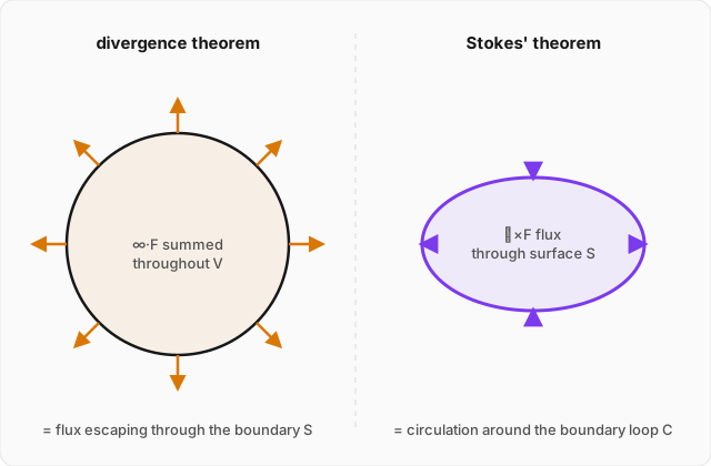
The second payoff connects a volume integral of divergence to a surface integral of flux, over the closed surface bounding that volume:

\oint_S \vec F\cdot d\vec A = \int_V (\nabla\cdot\vec F)\,dV.

Read it exactly as the meaning of divergence suggests it should be read: the left side is the total flux escaping through the boundary of a region; the right side is the sum, over every point inside, of how much of a "source" is sitting there. Total outflow equals total source strength — a statement so intuitive once divergence has been defined that the theorem almost proves itself; the actual work is in the details of the proof, which we won't carry out here, but the content of the result is exactly this bookkeeping statement.

Stokes' theorem

The third payoff plays the identical role for curl and circulation:

\oint_C \vec F\cdot d\vec l = \int_S (\nabla\times\vec F)\cdot d\vec A,

where $C$ is a closed loop and $S$ is any surface with $C$ as its boundary. The circulation of $\vec F$ all the way around a closed loop equals the total curl — total "local swirl" — passing through any surface stretched across that loop. The word "any" is worth pausing on: a wildly bulging surface and a flat one, both bounded by the same loop, give the identical flux of curl. That's a nontrivial, almost surprising fact, and it is exactly what the theorem guarantees.

Two panels. Left: a closed surface with outward-pointing flux arrows on its boundary, illustrating the divergence theorem — total flux out equals the divergence summed throughout the enclosed volume. Right: a closed loop with a bulging surface stretched across it and circulation arrows along the boundary, illustrating Stokes' theorem — circulation around the loop equals the curl's flux through the surface. — Both theorems say the same kind of thing: a local quantity (divergence, curl), summed over an entire region, exactly reproduces a global quantity (flux, circulation) measured only on that region's boundary.

Worked example

Verify the divergence theorem for $\vec F(x,y,z) = (x,y,z)$ on a sphere of radius $R$ centered at the origin, by computing both sides independently. (click to reveal the solution)

Setting up: we need $\int_V (\nabla\cdot\vec F)\,dV$ and $\oint_S \vec F\cdot d\vec A$ separately, for the same field and the same sphere, and check that they agree.

The volume side — computing the divergence first:

\nabla\cdot\vec F = \frac{\partial x}{\partial x}+\frac{\partial y}{\partial y}+\frac{\partial z}{\partial z} = 1+1+1 = 3.

The divergence is the constant $3$ everywhere, so the volume integral is just $3$ times the volume of the sphere:

\int_V (\nabla\cdot\vec F)\,dV = 3\int_V dV = 3\left(\frac{4}{3}\pi R^3\right) = 4\pi R^3.

The surface side — computing the flux directly: on the surface of the sphere, every position vector $\vec r=(x,y,z)$ has magnitude exactly $R$ , and points radially outward — which is also the direction of the outward normal $\hat n$ there. So on this particular surface, $\vec F = \vec r = R\hat n$ : the field is simply $R$ times the outward unit normal, at every point of the sphere.

The area element can be written $d\vec A = \hat n\, R^2\,d\Omega$ , where $d\Omega$ is an element of solid angle (this is the standard way to parametrize a sphere's surface — the full sphere spans solid angle $4\pi$ ). Then:

\vec F\cdot d\vec A = (R\hat n)\cdot(\hat n\,R^2\,d\Omega) = R^3(\hat n\cdot\hat n)\,d\Omega = R^3\,d\Omega,

using $\hat n\cdot\hat n=1$ since $\hat n$ is a unit vector. Integrating over the full sphere:

\oint_S \vec F\cdot d\vec A = R^3\int d\Omega = R^3(4\pi) = 4\pi R^3.

Comparing: both sides equal $4\pi R^3$ , exactly. The theorem holds, verified on a case simple enough to compute honestly by hand on both sides — which is the only way to actually trust a theorem like this rather than just accepting it on authority.

Where this leads

These two theorems — divergence and Stokes' — are not mathematical curiosities kept for their own sake. They are the precise machinery that converts physical laws back and forth between two equivalent forms: a local differential statement (true at every point separately) and a global integral statement (true over an entire region or loop at once). Electric charge creates an electric field whose divergence is proportional to charge density at every point — or, in exactly equivalent language via this theorem, whose total flux through any closed surface is proportional to the total charge enclosed. Both statements say the same physics; this topic is what lets you move freely between them. That move is about to become the entire content of Gauss's law, the next stop on the electromagnetism branch of this track.