The Biot-Savart Law and Ampère's Law

The previous topic told you what a magnetic field does — bends a moving charge's path, pushes on a current-carrying wire — without ever saying where a magnetic field actually comes from. Oersted's compass needle demands an answer: a current made that needle move, so a current must be creating a magnetic field around itself, the same way a charge creates an electric field around itself. What's the law?

The Biot-Savart law: building a field piece by piece

Split a current-carrying wire into infinitesimal segments $d\vec l$ , each carrying current $I$ . Just as a point charge $dq$ contributes a piece $dq/r^2$ to an electric field (Coulomb's law in differential form), each current element contributes a piece of magnetic field at a point displaced from it by $\vec r$ (with $\hat r$ the unit vector from the element to the field point):

d\vec B = \frac{\mu_0}{4\pi}\frac{I\,d\vec l\times\hat r}{r^2}.

This is the Biot-Savart law, and the constant $\mu_0\approx 4\pi\times10^{-7}\ \text{T}\cdot\text{m/A}$ (the permeability of free space) plays exactly the role $1/4\pi\epsilon_0$ played in Coulomb's law: a fixed conversion factor between the units chosen for current and the units chosen for field. Everything about the field's direction lives in the cross product $d\vec l\times\hat r$ — the field circles around the current element, perpendicular to both the wire and the line to the field point, never pointing straight at it the way an electric field does. That's the geometric fingerprint of magnetism: electric field lines start and end on charges; magnetic field lines wrap around currents in closed loops, with no beginning and no end.

Getting the total field at a point means integrating this contribution over the entire current distribution:

\vec B = \frac{\mu_0}{4\pi}\int \frac{I\,d\vec l\times\hat r}{r^2}.

This is completely general and always works, in principle. In practice it can be a brutal integral, exactly the way Coulomb's law's field integral can be brutal for a complicated charge distribution — which is precisely the situation that motivated Gauss's law as a shortcut for symmetric cases. Magnetism has the identical shortcut, built from the identical kind of idea.

Ampère's law: the magnetic analog of Gauss's law

Gauss's law rewrote Coulomb's law as a statement about flux through a closed surface, exploiting symmetry to skip the direct integral entirely. The magnetic analog exploits Stokes' theorem instead of the divergence theorem, and it relates not flux but circulation — the line integral of $\vec B$ around a closed loop — to the current passing through that loop:

\boxed{\oint \vec B\cdot d\vec l = \mu_0 I_{\text{enc}}.}

This is Ampère's law. $I_{\text{enc}}$ is the total current threading through any surface bounded by the closed loop $C$ you integrate around; it doesn't matter which surface you pick, bulging or flat, exactly as Stokes' theorem guarantees.

Here is where the derivation actually connects to something already built. Stokes' theorem says $\oint_C \vec F\cdot d\vec l = \int_S(\nabla\times\vec F)\cdot d\vec A$ for any vector field $\vec F$ . Apply it to $\vec B$ :

\oint_C \vec B\cdot d\vec l = \int_S (\nabla\times \vec B)\cdot d\vec A.

Meanwhile, the enclosed current can be written as the flux of the current density $\vec J$ through that same surface, $I_{\text{enc}} = \int_S \vec J\cdot d\vec A$ . Ampère's law in integral form, $\oint\vec B\cdot d\vec l = \mu_0 I_{\text{enc}}$ , therefore reads

\int_S(\nabla\times\vec B)\cdot d\vec A = \mu_0\int_S \vec J\cdot d\vec A.

Since this has to hold for every surface $S$ bounded by every possible loop $C$ — not just one convenient choice — the integrands themselves must agree at every point, giving the differential form:

\nabla\times\vec B = \mu_0\vec J.

Read this the same way divergence and curl taught you to read such an equation: current density is a local source of circulation for the magnetic field, exactly as charge density is a local source of divergence for the electric field in Gauss's law. Two completely parallel statements, one for each field, both proven the same way — a local differential law and a global integral law, connected by an integral theorem, exactly the machinery built for this purpose.

Two panels. Left: an infinite straight wire carrying current I out of the page's plane, surrounded by concentric circular field lines with arrows showing the circulation direction from the right-hand rule, and one circular Amperian loop of radius r drawn with B tangent to it everywhere. Right: a solenoid drawn in cross-section as a row of circular loops, with a dense uniform field of parallel arrows inside and a thin rectangular Amperian loop straddling the boundary, half inside and half outside the coil. — Ampère's law turns two hard integrals into easy algebra, once symmetry lets you pull the field strength outside the loop integral: a circular loop around a straight wire, and a rectangular loop straddling a solenoid's windings.

Worked example

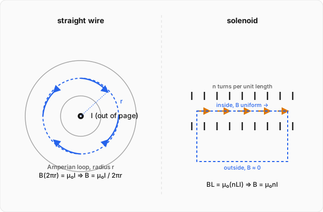
Use Ampère's law to find the magnetic field a distance $r$ from an infinite straight wire carrying current $I$ , and the field inside an ideal solenoid with $n$ turns per unit length carrying current $I$ . (click to reveal the solution)

Part 1 — the straight wire. Setting up: by the symmetry of an infinite straight wire, the field can only depend on the distance $r$ from the wire, and by the Biot-Savart law's cross product, it must circle the wire — so choose the Amperian loop to be a circle of radius $r$ centered on the wire, in the plane perpendicular to it. On this loop, $\vec B$ is tangent to the circle everywhere and has the same magnitude $B$ at every point on it, by symmetry.

Evaluating the circulation integral: because $\vec B$ is parallel to $d\vec l$ everywhere on this particular loop and constant in magnitude, it comes straight out of the integral:

\oint \vec B\cdot d\vec l = B\oint dl = B(2\pi r),

using the fact that $\oint dl$ around a circle of radius $r$ is just its circumference, $2\pi r$ .

Applying Ampère's law: the loop encloses the entire wire, so $I_{\text{enc}}=I$ , giving

B(2\pi r) = \mu_0 I \quad\Longrightarrow\quad \boxed{B = \frac{\mu_0 I}{2\pi r}.}

The field falls off as $1/r$ — not $1/r^2$ — a direct consequence of the geometry: field lines here are circles that grow in circumference, not spheres that grow in area.

Part 2 — the ideal solenoid. Setting up: an ideal solenoid is idealized as producing a uniform field $B$ inside, parallel to its axis, and (approximately) zero field outside. Choose a rectangular Amperian loop: one long side of length $L$ buried inside the solenoid, parallel to the axis; the opposite side of the same length $L$ , running parallel to it but outside the solenoid, where the field is taken to be zero; and two short sides connecting them, perpendicular to the field, contributing nothing to the circulation since $\vec B\cdot d\vec l=0$ there.

Evaluating the circulation integral piece by piece: the outside segment contributes zero ( $B=0$ there); each perpendicular segment contributes zero ( $\vec B\perp d\vec l$ ); only the inside segment survives, where $\vec B$ is uniform and parallel to $d\vec l$ :

\oint \vec B\cdot d\vec l = BL + 0 + 0 + 0 = BL.

Counting the enclosed current: the rectangular loop of length $L$ encloses $nL$ individual turns of wire (since there are $n$ turns per unit length), each carrying current $I$ , so

I_{\text{enc}} = nLI.

Applying Ampère's law:

BL = \mu_0 (nLI) \quad\Longrightarrow\quad \boxed{B = \mu_0 n I,}

with the length $L$ cancelling from both sides — as it must, since the loop's length was an arbitrary choice, and the physical field inside the solenoid can't depend on how long a loop we happened to draw. The result is uniform, independent of position inside an ideal (infinitely long) solenoid, and depends only on the turn density and the current — which is exactly why solenoids are the standard way to build a controllable, uniform laboratory magnetic field.

Where this leads

Ampère's law as written here — $\oint\vec B\cdot d\vec l=\mu_0 I_{\text{enc}}$ — is correct for steady, unchanging currents, and it will turn out to need one more piece before it's the complete story. But first, there's a second, independent way that magnetic fields connect to electric ones, running in the opposite direction: a changing magnetic field turns out to create an electric field, all on its own, with no charges required. That's Faraday's law, and it's the last ingredient needed before all of electricity and magnetism can be assembled into one unified set of equations.