Gravitational Waves | ScienceCorpus

Take a charge and shake it. Electromagnetic waves showed exactly what happens: the field can't rearrange itself instantly, the change propagates outward at $c$ , and what leaves the charge is a self-sustaining hand-off between $\vec E$ and $\vec B$ that carries energy away and never comes back. That is radio, and light, and X-rays. It all follows from the fact that Maxwell's equations, with the sources switched off, still support a wave.

Now take a mass and shake it.

The analogy is so obvious that it was made almost immediately, and it is essentially right. But it took a hundred years to confirm, and — this is the part worth being surprised by — Einstein himself changed his mind about whether gravitational waves existed at all. He predicted them in 1916, and then in 1936 submitted a paper with Nathan Rosen to Physical Review titled "Do Gravitational Waves Exist?", arguing that they do not. The referee report said the argument was wrong. Einstein, unused to anonymous refereeing, withdrew the paper in irritation and published a corrected version elsewhere. The referee, Howard Percy Robertson, had been right.

So this is not a case of an easy analogy carried across. Something genuinely different happens on the gravitational side, and the first thing to do is find out what.

Why the obvious analogy fails, and what replaces it

In electromagnetism, radiation is organized by multipole order. The monopole — total charge — cannot radiate, because charge is conserved: $\dot q = 0$ , so there is nothing to accelerate. The dipole

\vec d = \sum_i q_i\vec r_i

is where radiation starts, and it dominates everything: an antenna is a device for making $\ddot{\vec d}$ large.

Run the same argument for gravity, whose "charge" is mass-energy. The monopole is the total mass $M$ , conserved, so no monopole radiation — which we already knew from a completely different direction, since Birkhoff's theorem in the Schwarzschild solution says a spherically pulsating star produces a strictly static exterior metric. A radially breathing sphere radiates nothing at all. Now the dipole:

\vec d_{\text{grav}} = \sum_i m_i\vec r_i = M\vec R_{\text{cm}}.

Differentiate once:

\dot{\vec d}_{\text{grav}} = \sum_i m_i\vec v_i = \vec P_{\text{total}}.

And that is conserved. So

\ddot{\vec d}_{\text{grav}} = \dot{\vec P}_{\text{total}} = 0

identically, for any isolated system. Gravitational dipole radiation does not exist. The contrast with electromagnetism is sharp and instructive: there, $\sum q_i\vec v_i$ is not a conserved quantity, because charge and mass are independent properties and there is no conservation law protecting the charge-weighted momentum. In gravity, the "charge" is the mass, so the first derivative of the dipole moment is the total momentum, and momentum conservation kills the whole channel.

The leading order is therefore the quadrupole,

Q_{ij} = \sum_k m_k\left(x_k^ix_k^j - \tfrac{1}{3}\delta^{ij}r_k^2\right),

and radiation requires $\dddot{Q}_{ij}\neq 0$ . This is not a technicality. It is the reason gravitational waves are so faint, it dictates what kinds of source can produce them, and it explains why the loudest events in the universe are objects orbiting each other — a mass distribution that changes shape, not just position. A spinning perfectly axisymmetric object radiates nothing; a spinning dumbbell radiates.

Linearizing the field equations

The Einstein field equations are ten coupled nonlinear PDEs, and nothing about them looks like a wave equation. To find the waves, do what physics always does with an intractable nonlinear system: look for small disturbances about a known solution.

Take flat spacetime as the background and write

g_{\mu\nu} = \eta_{\mu\nu} + h_{\mu\nu}, \qquad |h_{\mu\nu}| \ll 1,

where $\eta_{\mu\nu}=\mathrm{diag}(-1,1,1,1)$ is the Minkowski metric from curved spacetime and the metric tensor and $h_{\mu\nu}$ is a small, symmetric perturbation — ten small functions of spacetime. Keep only terms linear in $h$ and discard everything quadratic and beyond.

Now the honest accounting of what happens next. Substituting this into $\Gamma$ , then into the Riemann tensor, then contracting to get $R_{\mu\nu}$ and $G_{\mu\nu}$ , expanding everything to first order in $h$ , and then exploiting the gauge freedom (the freedom to make small coordinate changes, which shuffles $h_{\mu\nu}$ around without changing the physics) to impose the Lorenz-like condition $\partial^\mu\bar h_{\mu\nu}=0$ on the trace-reversed perturbation $\bar h_{\mu\nu} \equiv h_{\mu\nu}-\tfrac12\eta_{\mu\nu}h$ — all of that is a long, careful, entirely mechanical computation. It uses the Riemann tensor formula which this track quoted rather than derived. I am not going to perform it here, and I am not going to pretend that the result below has been shown. What I will do is state it, and then verify that it behaves the way a wave equation must.

The result is

\Box\,\bar h_{\mu\nu} = -\frac{16\pi G}{c^4}\,T_{\mu\nu}, \qquad \Box \equiv \eta^{\mu\nu}\partial_\mu\partial_\nu = -\frac{1}{c^2}\frac{\partial^2}{\partial t^2} + \nabla^2.

Ten decoupled wave equations with sources — the coupling being twice that of the full field equations, a factor that comes out of the trace reversal. And in vacuum, where $T_{\mu\nu}=0$ , one can further specialize the gauge (the transverse-traceless or TT gauge) so that $h_{\mu\nu}$ is itself traceless, $\bar h_{\mu\nu}=h_{\mu\nu}$ , and

\boxed{\ \Box\, h_{\mu\nu} = 0 \qquad\Longleftrightarrow\qquad \frac{\partial^2 h_{\mu\nu}}{\partial t^2} = c^2\nabla^2 h_{\mu\nu}.\ }

Look at what that is. It is precisely the equation classical field theory derived from a Lagrangian density for a scalar field,

\partial_t^2\phi = v^2\partial_x^2\phi,

generalized from one spatial dimension to three and with $v$ replaced by $c$ — the same generalization electromagnetic waves made to reach $\nabla^2\vec E = \mu_0\epsilon_0\,\partial_t^2\vec E$ . Three completely different physical systems, one equation. The field being waved is different in each case — a displacement, an electromagnetic field, the metric of spacetime — but the mathematics does not care.

Solving it is therefore something we can do honestly and completely, because that page already established the method: guess a travelling cosine, differentiate twice, and see what the equation demands. Take a wave running along $z$ :

h_{\mu\nu}(z,t) = A_{\mu\nu}\cos(kz-\omega t),

with $A_{\mu\nu}$ a constant symmetric matrix of amplitudes. Two time derivatives:

\partial_t h_{\mu\nu} = A_{\mu\nu}\,\omega\sin(kz-\omega t), \qquad \partial_t^2 h_{\mu\nu} = -A_{\mu\nu}\,\omega^2\cos(kz-\omega t).

Two spatial derivatives (only $z$ appears, so $\nabla^2 \to \partial_z^2$ ):

\partial_z h_{\mu\nu} = -A_{\mu\nu}\,k\sin(kz-\omega t), \qquad \partial_z^2 h_{\mu\nu} = -A_{\mu\nu}\,k^2\cos(kz-\omega t).

Substituting into the boxed equation:

-A_{\mu\nu}\omega^2\cos(kz-\omega t) = c^2\left[-A_{\mu\nu}k^2\cos(kz-\omega t)\right].

Cancelling the common nonzero factor $-A_{\mu\nu}\cos(kz-\omega t)$ :

\omega^2 = c^2k^2 \qquad\Longrightarrow\qquad \boxed{\ \omega = ck.\ }

Gravitational waves travel at exactly the speed of light, for every wavelength, with no dispersion. Not "approximately $c$ ," not " $c$ in some limit" — the linearized field equations contain no other speed. (This is now measured, not just predicted: GW170817, a neutron-star merger, arrived $1.7$ seconds before its gamma-ray flash after $130$ million years of travel, pinning the fractional difference between the speed of gravity and the speed of light below about $10^{-15}$ .)

What the wave actually does

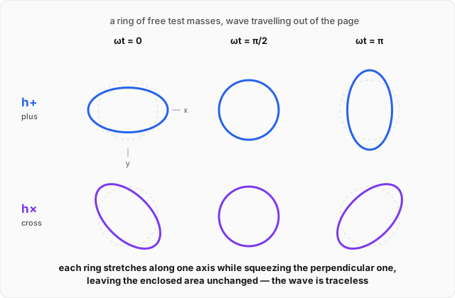
In TT gauge the ten components of $h_{\mu\nu}$ collapse dramatically. Transversality kills everything with a $z$ or $t$ index, tracelessness removes one more, and symmetry does the rest, leaving exactly two independent amplitudes for a wave travelling along $z$ :

h_{\mu\nu} = \begin{pmatrix} 0&0&0&0\\ 0&h_+&h_\times&0\\ 0&h_\times&-h_+&0\\ 0&0&0&0 \end{pmatrix} \cos(kz-\omega t).

Two polarizations, called plus and cross, exactly as an electromagnetic wave has two. And notice the $-h_+$ in the $yy$ slot: it is forced by tracelessness, and it is the whole physical signature of a gravitational wave. Whatever the wave does to the $x$ direction, it does the opposite to $y$ .

To see what that means with a ruler, use the metric. Two free test masses sit at rest, separated by a distance $L$ along $x$ . The proper distance between them is $\int\sqrt{g_{xx}}\,dx$ , and with $g_{xx} = 1+h_+$ ,

L_x = L\sqrt{1+h_+} \approx L\left(1+\tfrac{1}{2}h_+\right), \qquad L_y \approx L\left(1-\tfrac{1}{2}h_+\right).

So each arm stretches or squeezes by a fractional amount $\tfrac12 h_+$ , one arm growing while the perpendicular one shrinks, in antiphase, at the wave frequency. Half a period later they swap. The two directions together preserve area to first order — which is tracelessness, made visible.

This is why gravitational waves are described by a strain rather than a force or an amplitude: the quantity that matters is dimensionless, it is a fractional length change, and — crucially — the absolute displacement it produces is proportional to how long your ruler is. Doubling the length of your detector doubles the signal. That single fact is the reason LIGO's arms are $4$ kilometres long.

A two-row, three-column diagram showing a ring of free test masses deformed by a passing gravitational wave travelling out of the page. Each cell has a faint dashed reference circle. The top row, labelled h-plus, shows an ellipse stretched horizontally at phase zero, a circle at phase one quarter, and an ellipse stretched vertically at phase one half. The bottom row, labelled h-cross, shows the same three shapes rotated by forty-five degrees. A note beneath states that each ring stretches along one axis while squeezing the perpendicular one, leaving the area unchanged. — The two polarizations of a gravitational wave, shown as the deformation of a ring of freely floating test masses with the wave coming out of the page. The cross polarization is the plus polarization rotated by 45 degrees, not 90 — that halved angle is what a spin-2 field looks like, as against the 90 degrees separating an electromagnetic wave's two polarizations.

How large is $h$ , really?

The amplitude far from a source is given by the quadrupole formula (quoted, not derived — it requires solving the sourced equation above with a retarded Green's function):

h_{ij} \sim \frac{2G}{c^4 D}\,\ddot{Q}_{ij}\!\left(t-\frac{D}{c}\right),

with $D$ the distance to the source. That $G/c^4$ out front is the same catastrophically small coupling — $2.08\times10^{-43}\ \text{m}/\text{J}$ , computed in the Einstein field equations — that makes gravity weak in the first place. It is now standing between us and any hope of detection.

Estimate it for a binary of masses $M_1,M_2$ in a circular orbit of separation $d$ . The quadrupole moment is of order $\mu d^2$ with $\mu = M_1M_2/M$ the reduced mass, and it oscillates at the orbital frequency, so $\ddot Q\sim \mu d^2\omega^2$ . Kepler gives $\omega^2 = GM/d^3$ , hence

\ddot Q \sim \mu d^2\cdot\frac{GM}{d^3} = \frac{GM_1M_2}{d},

and dropping factors of order unity,

h \sim \frac{4G^2M_1M_2}{c^4\,d\,D} = \frac{4}{dD}\left(\frac{GM_1}{c^2}\right)\left(\frac{GM_2}{c^2}\right).

Written that way it is transparent: $h$ is the product of the two masses' gravitational radii divided by the orbital separation and the distance to us. Put in GW150914 — black holes of $36$ and $29$ solar masses, at a separation of a few hundred kilometres just before merger, at $410\ \text{Mpc} = 1.27\times10^{25}\ \text{m}$ :

\frac{GM_1}{c^2} = 5.3\times10^4\ \text{m}, \qquad \frac{GM_2}{c^2} = 4.3\times10^4\ \text{m}, \qquad d\approx 3.5\times10^5\ \text{m},

h \sim \frac{4(5.3\times10^4)(4.3\times10^4)}{(3.5\times10^5)(1.27\times10^{25})} = \frac{9.1\times10^{9}}{4.4\times10^{30}} = 2\times10^{-21}.

The measured peak strain was $1.0\times10^{-21}$ . A crude estimate with all the $O(1)$ factors thrown away, landing within a factor of two — which is exactly what such an estimate is entitled to, and no more.

The detections

Indirect, 1974. Russell Hulse and Joseph Taylor found a pulsar in a binary orbit, PSR B1913+16, and used its pulse timing as a clock of extraordinary precision. General relativity predicts such a system must lose energy to gravitational radiation and spiral inward, shortening its orbital period at a calculable rate. It does, and the measured decay matches the quadrupole prediction to better than a percent, over decades. Nobel Prize, 1993. After that, essentially nobody doubted gravitational waves existed; the question was whether one could be caught in the act.

Direct, 2015. On 14 September 2015 the two LIGO detectors, in Louisiana and Washington, both recorded a signal sweeping upward in frequency from $35$ to $250\ \text{Hz}$ over about $0.2\ \text{s}$ and then cutting off — the last few orbits and merger of two black holes, $1.3$ billion light years away. The event radiated about $3$ solar masses of energy as gravitational waves,

E \approx 3M_\odot c^2 = 5.4\times10^{47}\ \text{J},

with a peak luminosity of roughly $3.6\times10^{49}\ \text{W}$ — which, for a couple of hundredths of a second, exceeded by more than an order of magnitude the combined light output of every star in the observable universe. Announced February 2016; Nobel Prize 2017. Since then such detections have become routine, numbering in the hundreds.

And the thing that reached Earth from that titanic event, after travelling for $1.3$ billion years, was a fractional stretching of space of one part in $10^{21}$ . What that means for a real instrument is the subject of the worked example.

Worked example

LIGO measured a peak strain $h = 1.0\times10^{-21}$ with arms of length $L = 4.0\ \text{km}$ . Find the resulting change in arm length and compare it to something physical. Then work out whether the measurement is even possible in principle: compute the optical phase shift it produces and the laser power needed to resolve that phase against photon shot noise. (click to reveal the solution)

Setting up, and a factor of two worth getting right. LIGO quotes strain as the differential fractional arm-length change,

h = \frac{\Delta L}{L}, \qquad \Delta L \equiv \delta L_x - \delta L_y,

which is what an interferometer measures. From the metric analysis above, a plus-polarized wave arriving along the axis perpendicular to both arms gives $\delta L_x = +\tfrac12 hL$ and $\delta L_y = -\tfrac12 hL$ , so each individual arm moves by half of $\Delta L$ and the two move oppositely.

Differential length change:

\Delta L = hL = (1.0\times10^{-21})(4.0\times10^{3}\ \text{m}) = 4.0\times10^{-18}\ \text{m},

with each arm changing by $2.0\times10^{-18}\ \text{m}$ .

What sort of a length is that? Compare with a proton's charge radius, $0.84\times10^{-15}\ \text{m}$ :

\frac{\Delta L}{r_p} = \frac{4.0\times10^{-18}}{8.4\times10^{-16}} = 4.8\times10^{-3} \approx \frac{1}{210}.

A four-kilometre steel-and-glass instrument, measuring a length change of one two-hundredth of the radius of a proton. Compared with an atom ( $\sim10^{-10}\ \text{m}$ ) it is $4\times10^{-8}$ of an atomic diameter. Stated that way it sounds impossible, and it is worth understanding why it is not: the mirror surface is not a single atom. LIGO's beam has a radius of about $6\ \text{cm}$ , so it illuminates an area of $\pi(0.06\ \text{m})^2 = 1.1\times10^{-2}\ \text{m}^2$ ; with fused silica's atomic spacing of $3.6\times10^{-10}\ \text{m}$ that is of order $10^{17}$ atoms, and the laser measures the average position of all of them. Individual atoms jitter thermally by vastly more than $10^{-18}\ \text{m}$ ; the mean of $10^{17}$ of them does not.

Now the optical phase. LIGO's laser has wavelength $\lambda = 1064\ \text{nm}$ , and each arm is a Fabry-Perot cavity in which the light makes roughly $N\approx 300$ round trips before leaving, multiplying the effective path length by that factor. The differential round-trip path change is therefore

\Delta s = 2N\,\Delta L = 2(300)(4.0\times10^{-18}\ \text{m}) = 2.4\times10^{-15}\ \text{m},

the factor of $2$ being out-and-back. The corresponding phase difference at the beam splitter is

\Delta\phi = \frac{2\pi\,\Delta s}{\lambda} = \frac{2\pi(2.4\times10^{-15})}{1.064\times10^{-6}} = 2\pi(2.26\times10^{-9}) = 1.4\times10^{-8}\ \text{rad}.

Fourteen nanoradians. Nine orders of magnitude below the wavelength-scale phase shifts a classroom interferometer resolves by eye.

Is that measurable at all? The fundamental limit is photon counting. Light arrives in discrete quanta, so the number detected in a measurement interval fluctuates by $\sqrt{N_{\text{ph}}}$ about its mean (Poisson statistics), which translates into a phase uncertainty

\Delta\phi_{\min}\approx\frac{1}{\sqrt{N_{\text{ph}}}}.

Setting $\Delta\phi_{\min} = \Delta\phi$ and solving for the number of photons required:

N_{\text{ph}} = \frac{1}{(\Delta\phi)^2} = \frac{1}{(1.417\times10^{-8})^2} = \frac{1}{2.01\times10^{-16}} = 5.0\times10^{15}.

Five thousand million million photons. But over what time? The signal was in the $35$ – $250\ \text{Hz}$ band, so a single cycle near $100\ \text{Hz}$ lasts about $\tau = 0.01\ \text{s}$ . The required photon rate is

\frac{N_{\text{ph}}}{\tau} = \frac{5.0\times10^{15}}{0.01\ \text{s}} = 5.0\times10^{17}\ \text{photons/s}.

Each photon at $1064\ \text{nm}$ carries

E_\gamma = \frac{hc}{\lambda} = \frac{(6.626\times10^{-34})(2.998\times10^{8})}{1.064\times10^{-6}} = 1.87\times10^{-19}\ \text{J},

so the required optical power is

P = (5.0\times10^{17}\ \text{s}^{-1})(1.87\times10^{-19}\ \text{J}) = 0.093\ \text{W} \approx 0.1\ \text{W}.

Interpretation. A tenth of a watt. Roughly a laser pointer. That is the entire answer to "how can anyone possibly measure $10^{-18}$ metres" — and it is a genuinely surprising answer, because it says the quantum limit was never the obstacle. Advanced LIGO circulates about $100\ \text{kW}$ in each arm cavity, six orders of magnitude more power than this estimate demands, which buys a correspondingly enormous margin in phase resolution: shot noise falls as $1/\sqrt{P}$ , so a million times the power gives a thousand times better phase sensitivity.

The real obstacles are everything else, and they are all classical. Seismic motion — trucks, ocean waves, tectonic creep — moves the ground by around $10^{-9}\ \text{m}$ at the frequencies of interest, some nine orders of magnitude more than the signal, which is why the test masses hang from quadruple pendulum suspensions on actively controlled platforms. Thermal noise vibrates the mirror coatings. Residual gas molecules crossing the beam change the optical path, which is why the $4\ \text{km}$ tubes are pumped down to about $10^{-9}\ \text{torr}$ — roughly a trillionth of atmospheric pressure — making them among the largest vacuum systems on Earth. Detecting a gravitational wave was never a problem of insufficient light; it was a fifty-year engineering campaign against every other way a mirror can move.

And a last check on the physics: two detectors $3000\ \text{km}$ apart both saw GW150914, with the Louisiana detector recording it $6.9\ \text{ms}$ before the Washington one. A light-travel time between them is $3000\ \text{km}/c = 10\ \text{ms}$ , so a $6.9\ \text{ms}$ offset is consistent with a signal crossing the Earth at $c$ from a particular direction in the sky — which is both a sky-localization measurement and an independent confirmation of the $\omega=ck$ derived above.

Where this leads

This is the end of the general relativity track, and it is worth looking back at what the chain actually did. It started with a numerical coincidence Newton could not explain — that $m_g=m_i$ — and ended with an instrument measuring a thousandth of a proton's width to confirm a wave equation. Every link was forced by the one before it. The equivalence principle demanded that gravity be locally erasable, which forced curved spacetime; curvature demanded a law of motion, which turned out to be the geodesic equation and, hiding inside it, the principle of least action from Lagrangian mechanics; a law of motion demanded a field equation, which is Einstein's; the field equations, solved exactly, gave black holes, and linearized, gave the waves on this page.

Gravitational waves are also the point where general relativity becomes an observational instrument rather than a theory being tested. Light has told us about the universe for four hundred years, but light is emitted by the surfaces of things and is absorbed by dust and gas. Gravitational waves are emitted by mass distributions in bulk and pass through everything essentially unattenuated, which means they carry information out of places light cannot leave: the interiors of collapsing stars, the merger of two horizons, and in principle the first fraction of a second of the universe, from before it was transparent to light at all.

One deep question this track cannot answer is what gravitational waves are made of. Classical field theory showed that any classical field decomposes into oscillator modes, and that quantizing one such mode gives a ladder of identical quanta — which is how the electromagnetic wave derived in electromagnetic waves becomes a stream of photons in quantum field theory. Applying the same construction to $h_{\mu\nu}$ ought to give a quantum of gravity, and the $45^\circ$ rather than $90^\circ$ structure of the two polarizations in the figure above says it would carry spin $2$ rather than spin $1$ . But that programme does not work: unlike every other field on this site, the quantized version of general relativity produces infinities that cannot be absorbed by redefining finitely many constants. Reconciling the geometry built in this track with the quantum mechanics built in the other is the outstanding unsolved problem in fundamental physics, and there is currently no experiment anywhere near probing it.

So the track ends where honesty requires it to: with a theory whose predictions for the double pulsar J0737 $-$ 3039 agree with observation to better than one part in ten thousand, which is load-bearing in the satellite navigation system in your pocket, and which is nonetheless known to be incomplete.