Game Theory and Oligopoly

Harbor Falls sits on a ridge of good hard rock, and two quarries work it: Northgate, on the inland side, and Slate Point, out by the water. Between them they supply every tonne of crushed stone the county's road program buys. Once a year the manager at Northgate has to decide how much to blast, and one autumn she sat down with a spreadsheet to do it properly.

She knew her costs cold: 30 dollars a tonne, near enough constant, for drilling, crushing, and hauling. She knew the demand side too, because the county publishes its bid schedules — across the whole market, price and quantity move together along $P = 150 - Q$, with $Q$ measured in thousands of tonnes a year and $P$ in dollars a tonne. So she wrote down the thing she wanted to maximize, which is revenue minus cost on her own output $q_N$:

And there the spreadsheet stopped, because of the $q_S$. Her profit depends on Slate Point's tonnage, and she does not know it. Worse, she knows why she does not know it: Slate Point's manager is at that same moment sitting at his own desk with the same demand curve and the same problem, and the number he is missing is hers. The calculation has a hole in the middle of it, and the only thing that fits the hole is another copy of the same calculation.

This is a genuinely new difficulty, and it is worth seeing that it is new rather than merely harder. In perfect competition a firm's rivals appear in its problem only through the market price, which it takes as given — there are so many of them that no one's decision is worth watching, and "what will the others do" is answered by a single posted number. In monopoly the difficulty vanishes for the opposite reason: there is nobody else, so the firm's own quantity determines the price outright, and $MR = MC$ closes the problem in one line. Both extremes have the same convenient property. A firm can solve its own optimization without ever modelling anyone else's mind.

Everything in between loses that property, and almost every real industry is in between. Two quarries, four airlines, three mobile networks, a dozen supermarket chains — in every one of these an oligopoly, a market with few enough sellers that each one's choices visibly move the outcome, the manager's problem contains a term she can only fill in by reasoning about somebody who is reasoning about her. Ordinary optimization has no machinery for that. It needs a language built for it, and this topic is about that language and what it says when you point it at Northgate and Slate Point.

You have used the language once already without being told its name. In public goods and common resources the crab boats in the bay each chose how many traps to set, each one's catch depending on everybody's traps, and the phrase "Nash equilibrium" was used to describe where they ended up. We will come back to that bay before the end and discover that it is, algebraically, the very same problem as the two quarries — which is a good sign that the language is worth learning properly rather than borrowing informally.

The elements of a game

Strip the quarry problem down to what is actually essential and you get three ingredients. Together they are a game.

Players. The decision-makers whose choices interact. Here, Northgate and Slate Point. In the bay, four crab boats. In the levee story, three neighborhoods. Nature can be a player too when there is genuine randomness, but we will not need her.

Strategies. The complete list of what each player might do. For Northgate the strategy set is every tonnage she might blast — a continuum, $q_N \ge 0$. For a game of two prisoners it is the two-element set {stay silent, confess}. The strategy set can be small and discrete or large and continuous; nothing in the theory cares.

Payoffs. A number attached to every combination of strategies, one number per player. This is where the interaction lives: a payoff is not a function of your own move, it is a function of the whole profile of moves. Northgate's payoff function is the $\pi_N$ written above, and it takes two arguments even though Northgate controls only one of them.

When there are two players with finitely many strategies each, all of this fits in a table — the normal form, or payoff matrix. Rows are player 1's strategies, columns are player 2's, and each cell holds the pair (player 1's payoff, player 2's payoff), row player first. The convention is worth being fussy about, because half the mistakes people make reading these tables are mistakes about which number belongs to whom.

Let us build one from the quarries by pretending, temporarily, that each manager must choose one of just three tonnages: 30, 40, or 55. Profit is

where the second form absorbs the marginal cost and is the one to compute with. Filling in all nine cells — for instance the (40, 55) cell gives Northgate $(120 - 40 - 55)(40) = 25 \times 40 = 1000$ and Slate Point $25 \times 55 = 1375$ — produces

in thousands of dollars a year. Every entry is one multiplication; check a couple yourself, because the whole of the next two sections is read off this table.

Dominance

The first question to ask of any game is whether some strategy is simply never worth playing. Strategy $s_i$ strictly dominates $s_i'$ for player $i$ if it yields a strictly higher payoff against every possible choice by the others:

where $s_{-i}$ is the standard shorthand for "everybody's strategy but $i$'s". A strictly dominated strategy is one a rational player will never use, and — this is the important part — you do not need to know anything at all about what the opponent will do to reach that conclusion. It is the one prediction game theory can make without any assumption about beliefs.

Read down the columns of the table for Northgate. Compare the row $q_N = 55$ with the row $q_N = 40$: against 30, $2000 > 1925$; against 40, $1600 > 1375$; against 55, $1000 > 550$. Blasting 55 is worse than blasting 40 no matter what Slate Point does, so 55 is strictly dominated and can be crossed out. By symmetry the same is true of Slate Point's column $q_S = 55$.

Now the subtle part, and the reason the procedure has the word iterated in its name. In the full table, does 40 dominate 30 for Northgate? Against $q_S = 30$: $2000 > 1800$, yes. Against $q_S = 40$: $1600 > 1500$, yes. Against $q_S = 55$: $1000 < 1050$ — no. If Slate Point were to flood the market with 55, Northgate would rather hold back to 30 than push to 40. So in the original game 30 survives.

But 55 has just been eliminated. If Slate Point is rational, Slate Point will never play 55, and Northgate — knowing Slate Point is rational — can delete that column before choosing. In the reduced 2×2 game on {30, 40}, the comparison against 55 no longer exists, and now $2000 > 1800$ and $1600 > 1500$ leave 40 strictly dominating 30. Delete 30 for both players and one cell remains:

That procedure is iterated elimination of strictly dominated strategies, and notice exactly what it assumed at each round. Round one needed only that each player is rational. Round two needed each player to be rational and to know the other is rational. A third round would need each to know that the other knows, and so on — the assumption stack that game theorists call common knowledge of rationality. It is a strong assumption and worth flagging as one; it is also, in this game, enough to pin down a unique prediction.

Two warnings. First, eliminating only strictly dominated strategies is safe, in that the order of elimination never changes the answer and no equilibrium is ever destroyed. Eliminating weakly dominated ones — where the inequality is $\ge$ with strictness somewhere — is not safe: the outcome can depend on the order you delete things in. Second, most games have no dominated strategies at all, and the procedure stops immediately without saying anything. We got lucky here. For the general case we need a different idea.

Nash equilibrium

Here is the idea, and it is worth stating carefully because its precision is the whole of its value.

A strategy profile $(s_1^*, s_2^*, \dots, s_n^*)$ is a Nash equilibrium if, for every player $i$, $u_i(s_i^*, s_{-i}^*) \ge u_i(s_i, s_{-i}^*) \quad\text{for all } s_i.$ That is: given what everyone else is doing, no player can do strictly better by changing their own strategy alone.

Three things this definition does not say, each of which is a standard misreading.

It does not say the outcome is good. Nothing in the definition mentions total payoffs, efficiency, or fairness. It is entirely possible — and the next subsection makes it happen — for every player to be worse off at the Nash equilibrium than at some other profile they could all have agreed on.

It does not say players cooperate or conspire. The test is unilateral: hold everyone else fixed and ask whether this one player wants to move. Joint deviations by two players at once are not considered, which is precisely why a Nash equilibrium can be beaten by a coalition.

It does not require anyone to be clever. It is a consistency condition on a profile, not a story about how anyone found it. A Nash equilibrium is a rest point: a configuration of behavior which, once reached, no individual has a reason to disturb.

The practical way to find one is by best responses. Define player $i$'s best-response correspondence $BR_i(s_{-i})$ as the set of strategies maximizing $u_i$ against $s_{-i}$. Then a profile is a Nash equilibrium exactly when every player's strategy is a best response to the others' — the equilibrium is the mutual fixed point of the best-response map. In a payoff table you find these mechanically: for each column, mark the row player's largest payoff; for each row, mark the column player's largest; any cell marked twice is an equilibrium.

Do it on the 3×3 quarry table. Column $q_S = 30$: Northgate's payoffs are 1800, 2000, 1925 — mark 2000, in row 40. Column $q_S = 40$: 1500, 1600, 1375 — mark 1600, row 40. Column $q_S = 55$: 1050, 1000, 550 — mark 1050, row 30. By symmetry Slate Point's marks fall in the mirror-image cells. The only cell marked by both is $(40, 40)$. Same answer as iterated dominance gave, which is not a coincidence: when iterated elimination of strictly dominated strategies leaves exactly one profile, that profile is the unique Nash equilibrium.

The prisoner's dilemma, and why a Nash equilibrium can be terrible

Take the 3×3 table and keep only the rows and columns 30 and 40:

Look at what this says. Expanding strictly dominates restraining, for both quarries: $2000 > 1800$ and $1600 > 1500$. So both expand, and each earns 1600. But if both had restrained, each would have earned 1800. Both players would be better off — strictly, by 200 thousand dollars a year each — at a profile that neither will play.

That is a prisoner's dilemma, and it is worth being exact about what makes it one, because the name gets thrown at any situation where people fail to cooperate. The defining structure is: defection strictly dominates cooperation for every player, and the all-defect profile is Pareto-dominated by the all-cooperate profile. Both halves matter. The first makes the bad outcome inevitable for rational players; the second makes it bad.

And now the sentence that carries the whole idea: the Nash equilibrium $(40, 40)$ is Pareto-inefficient. There exists another outcome that both players strictly prefer. This is not a paradox, a failure of the equilibrium concept, or evidence that people are stupid. It is a completely consistent state of affairs, because "both would prefer it" and "neither will unilaterally move toward it" are different claims, and Nash equilibrium only ever tests the second.

You have met this exact structure before. In public goods and common resources, four crab boats agreed in the harbor bar to set a thousand traps each, worth 400 thousand dollars apiece, and then any one of them could jump to 2,500 traps and make 625 while knocking the other three down to 250. Everyone saw the arithmetic, everyone defected, and the bargain never survived a season. That was a four-player prisoner's dilemma with a continuous strategy set, and it is the same object as the table above. The rest of this topic is largely about generalizing it: first to a continuum of quantities, then to prices, then to time.

One more remark before we do. Nash equilibria need not be unique, and in some games none exists in the pure strategies we have been using — the children's game of matching pennies has no rest point, because whatever the pair of choices, one player wants to switch. Nash's 1950 theorem is that if players may randomize (choose a mixed strategy, a probability distribution over their pure strategies), then every finite game has at least one equilibrium. The proof is a fixed-point argument: the best-response map takes the compact convex set of mixed-strategy profiles into itself, and Kakutani's theorem does the rest. We will not need mixing in what follows, but the existence result is why the concept is usable at all.

Cournot competition: choosing quantities

Now take away the artificial three-item menu and let the quarries choose any tonnage they like. This is the model Antoine Augustin Cournot published in 1838 — thirty-eight years before the marginal revolution and more than a century before Nash — and it is startling how completely he got there first.

Setup. Inverse demand $P = a - bQ$ with $Q = q_1 + q_2$; both firms have constant marginal cost $c$, with $a > c$ so that production is worth doing at all; each chooses its quantity, once, simultaneously, knowing the demand curve and each other's costs. Firm 1's payoff is

Firm 1's best response. Maximize over $q_1$, treating $q_2$ as a fixed number — that is exactly what the unilateral test in the Nash definition instructs us to do:

and $\dfrac{\partial^2 \pi_1}{\partial q_1^2} = -2b < 0$, so this stationary point really is the maximum. (If the formula returns a negative number — which happens when $q_2 > (a-c)/b$, the rival alone flooding the market past the competitive quantity — the true best response is $q_1 = 0$. It will not bind in what follows.)

That expression deserves a sentence of interpretation before we solve anything. Read it as: firm 1 behaves like a monopolist on the part of the demand curve its rival has left standing. Set $q_2 = 0$ and it gives $q_1 = (a-c)/2b$, the monopoly quantity exactly. Every unit the rival produces knocks half a unit off firm 1's own output — the slope is $-1/2$, not $-1$ — so the firms partly, but only partly, offset each other. That partial offset is why the industry ends up somewhere strictly between monopoly and competition rather than at either end.

Equilibrium. Firm 2's best response is the mirror image, $q_2 = (a - c - bq_1)/2b$. A Nash equilibrium is a pair where each is a best response to the other, so substitute one into the other:

Collect the $q_1$ terms: $\tfrac34 q_1 = \tfrac{a-c}{4b}$, so

and by the symmetry of the two equations $q_2^* = q_1^*$, giving

We could have imposed symmetry at the start — set $q_1 = q_2 = q$ in the best-response function and solve $q = (a - c - bq)/2b \Rightarrow 3bq = a - c$ — but that would have assumed the equilibrium is symmetric rather than shown it. Doing it the long way costs three lines and proves there is no asymmetric solution: two linear equations with slopes $-1/2$ and $-2$ cross exactly once.

Put the quarry numbers in: $a = 150$, $b = 1$, $c = 30$, so $a - c = 120$.

Which is exactly the cell that iterated dominance picked out of the 3×3 table — a satisfying check, since the table only ever offered three tonnages and one of them happened to be right.

Three points on one line

Now put the answer next to the two cases we already know, using the same demand curve and the same cost so the comparison is honest.

Three fractions with the same numerator: $\tfrac12$, $\tfrac23$, $1$. The whole story of industrial organization is the claim that a real industry sits somewhere on that line, and the Cournot model says where.

The surplus column is computed the way consumer and producer surplus taught. Total surplus at quantity $Q$ is the area under demand minus the resource cost,

maximized at $Q = 120$ with $TS = 7200$; at $Q = 80$ it is $9600 - 3200 = 6400$, and at $Q = 60$ it is $7200 - 1800 = 5400$. So duopoly destroys $7200 - 6400 = 800$ thousand dollars a year of value and monopoly destroys $1800$. Cross-check each as a triangle with base $120 - Q$ and height $P - c$: $\tfrac12(40)(40) = 800$ and $\tfrac12(60)(60) = 1800$. ✓ Adding one rival cut the deadweight loss by more than half. Not to zero — a duopoly is not a competitive market — but competition is not an on/off switch, and the second firm did most of the work.

Look also at the industry profit column, which falls from 3600 to 3200. The two firms jointly would rather be a monopoly. They cannot get there by each choosing quantities independently, and that tension is the seed of the collusion section below.

Why the markup shrinks: $n$ firms

Nothing in the derivation cared that there were two firms. With $n$ symmetric firms, firm $i$ maximizes $\pi_i = \left[a - b\left(q_i + Q_{-i}\right)\right]q_i - c q_i$ where $Q_{-i}$ is everybody else's total, and the first-order condition is

The equilibrium is symmetric (same argument as before: the system is linear and has a unique solution), so put $q_i = q$ and $Q_{-i} = (n-1)q$:

Check the two cases we have: $n = 1$ gives $\tfrac12 \cdot \tfrac{a-c}{b}$, the monopoly quantity ✓, and $n = 2$ gives $\tfrac23 \cdot \tfrac{a-c}{b}$ ✓. And as $n \to \infty$ the factor $\tfrac{n}{n+1} \to 1$, so $Q^* \to \tfrac{a-c}{b}$, the perfectly competitive quantity. The price follows:

The markup over marginal cost decays like $1/(n+1)$ and each firm's profit like $1/(n+1)^2$. In the quarry numbers:

Read the markup column and you get a fact that is worth more than the model that produced it: the first few entrants do nearly all the work. Going from one firm to two cuts the markup by a third; going from five to ten cuts it by less than half again, and every firm after that matters less than the one before. This is why competition authorities fight hardest over mergers that take an industry from three players to two, and why an industry with fifty firms is treated as competitive without anyone checking further.

There is a bridge here to the monopoly topic that is exact rather than rhetorical. The Lerner index defined there, $L = (P - c)/P$, equals $1/|\varepsilon|$ for a monopolist. For $n$ symmetric Cournot firms it equals

where $\varepsilon$ is the market demand elasticity at the equilibrium. Verify it on the duopoly: $|\varepsilon| = \left|\tfrac{dQ}{dP}\right|\tfrac{P}{Q} = 1 \times \tfrac{70}{80} = 0.875$, so $\tfrac{1}{n|\varepsilon|} = \tfrac{1}{2 \times 0.875} = \tfrac{4}{7}$, while directly $\tfrac{P-c}{P} = \tfrac{40}{70} = \tfrac47$. ✓ Monopoly's formula is the $n=1$ case, and the competitive $P = MC$ is the $n \to \infty$ case. One equation covers the entire spectrum.

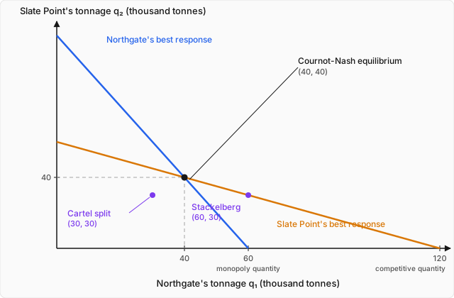
The diagram makes the failure of collusion geometrically obvious. The cartel point $(30, 30)$ lies below and to the left of both best-response lines. Sitting there, Northgate's best response to $q_S = 30$ is $R_1(30) = (120 - 30)/2 = 45$ — the arrow points right, away from the cartel. Slate Point's arrow points up. Only where the two lines cross does neither arrow point anywhere.

Bertrand competition: choosing prices

Cournot assumed firms choose quantities and let the market find a price. Joseph Bertrand, reviewing Cournot in 1883, objected that firms mostly do the opposite: they post prices, and sell whatever comes. Change that one assumption, keep everything else — identical product, identical constant marginal cost $c$, no capacity limits, simultaneous choice — and the answer changes completely.

The demand rule is now discontinuous, which is the whole story. Buyers see two identical goods and buy the cheaper one, so with $D(P) = (a - P)/b$ the market demand,

Claim: the unique Nash equilibrium is $P_1 = P_2 = c$, with zero profit for both. The proof is a sweep through the cases, and each case is a one-line unilateral deviation.

Case 1: $P_1 = P_2 = P > c$. Each firm earns $\tfrac12(P - c)D(P)$. Let firm 1 cut its price to $P - \epsilon$ for a tiny $\epsilon$. It now earns $(P - \epsilon - c)D(P-\epsilon)$, which as $\epsilon \to 0$ approaches $(P-c)D(P)$ — twice what it was making. For small enough $\epsilon$ it is strictly better off, so this is not an equilibrium. This is the step to sit with: shaving a hundredth of a cent off the margin buys the entire market. A vanishing cost buys a discrete gain, so there is no $\epsilon$ small enough to make undercutting unattractive, and therefore no price above $c$ at which the logic comes to rest.

Case 2: $P_1 > P_2 > c$. Firm 1 sells nothing and earns zero; it would rather set $P_1 = P_2 - \epsilon$ and earn something positive. Not an equilibrium.

Case 3: $P_1 > P_2 = c$. Firm 2 earns zero. It would rather raise its price to anything strictly between $c$ and $P_1$, capturing the whole market at a positive margin. Not an equilibrium.

Case 4: either price below $c$. The firm selling at that price makes a loss on every unit and would rather price at $c$ and sell nothing. Not an equilibrium.

Case 5: $P_1 = P_2 = c$. Each earns zero. Cutting price means selling at a loss; raising it means selling nothing, which also earns zero. No strictly profitable deviation exists, so this is an equilibrium — and by the elimination above, the only one. $\blacksquare$

The conclusion is the Bertrand paradox: two firms are enough to produce the perfectly competitive outcome. With our numbers, $P = 30$, $Q = 120$, zero profit, zero deadweight loss — the bottom row of the comparison table, reached with two sellers rather than infinitely many. Set that against Cournot's $P = 70$ with the same two firms and the same costs, and the size of the disagreement is alarming. Same industry, same technology, same number of firms; one model says the price is 70 and the other says 30.

Which is right? Both, and the honest answer is that the models differ in an assumption neither of them advertises: what a firm can commit to. A Cournot firm commits to a quantity and cannot serve more than it made; a Bertrand firm commits to a price and implicitly promises to serve everyone who shows up. The second promise is a strong one, and three ordinary features of real markets break it.

Capacity constraints. If each quarry can produce at most 50 thousand tonnes, undercutting no longer captures the market — it captures 50 thousand tonnes and leaves the rest to the rival, who can then charge what the residual demand will bear. Kreps and Scheinkman showed in 1983 that if firms first choose capacities and then compete in prices, the equilibrium outcome is exactly Cournot's. The quantity model is best understood not as a claim that firms choose quantities rather than prices, but as a reduced form for price competition between firms that had to build capacity first.

Product differentiation. Northgate's stone is closer to the county's northern roads; Slate Point's is closer to the harbor. Once the goods are not perfect substitutes, demand stops being a step function and becomes a smooth downward-sloping curve for each firm, undercutting by a cent wins a few marginal customers rather than all of them, and equilibrium prices settle strictly above marginal cost — rising with how differentiated the goods are.

Repetition. The undercutting argument is a one-shot argument. It says that today's gain from cutting exceeds today's loss. It says nothing about tomorrow, and that omission turns out to be the model's biggest.

Repeated games: how collusion becomes possible

Return to the prisoner's dilemma table. Both quarries would rather be at $(30, 30)$ earning 1800 than at $(40, 40)$ earning 1600, and no amount of talking fixes it, because talk does not change payoffs — an agreement to restrain is not a strategy, it is a wish about someone else's strategy.

But quarries do not shut down after one year. They meet the same rival, in the same market, next year and the year after. And a decision that is optimal today can be a mistake once the future's response is priced in. Making that precise requires two ingredients.

A discount factor. Write $\delta \in [0,1)$ for the value today of a dollar received one period from now. It bundles the interest rate — $\delta = 1/(1+r)$ — with the probability the relationship continues at all: if there is a chance $\rho$ each period that the county switches to imported aggregate and the game ends, then $\delta = \rho/(1+r)$. A patient, stable relationship has $\delta$ near 1; a one-off deal has $\delta = 0$. The present value of getting $\pi$ every period forever is the geometric sum

A strategy that responds to history. In a repeated game a strategy is not a single move; it is a rule assigning a move to every possible history of play. The simplest such rule with teeth is the grim trigger:

Produce the cartel quantity 30 in period 1, and in every later period produce 30 as long as both firms have produced 30 in every past period. If anyone has ever deviated, produce the Cournot quantity 40 forever after.

Now compute, for a firm considering whether to obey it while the rival does. Three numbers are needed and all three are already in hand:

The deviation payoff is not 2000, the number in the 2×2 table — that table only offered the tonnage 40. A firm that is going to be punished forever anyway should deviate optimally, so it plays its true best response to $q_S = 30$:

The condition. Colluding forever is worth

while deviating today and eating the punishment from tomorrow on is worth

Collusion is sustainable when $V^C \ge V^D$. Multiply through by $(1-\delta) > 0$:

The right-hand side is the one-off temptation divided by the total gap between temptation and punishment, which is exactly the trade-off stated in words. For the quarries:

So if the two managers value next year's dollar at more than about 53 cents, the cartel holds together with no contract, no enforcement, and no communication beyond both understanding the rule. Below that, it collapses to Cournot. Sanity-check the extremes: at $\delta = 0$ the condition fails and the firm defects, which must be right, since a firm with no future is playing a one-shot prisoner's dilemma; as $\delta \to 1$ the condition holds easily.

Three things fall out of the formula that are worth more than the number.

Harsher punishment sustains more collusion. Suppose deviation triggers Bertrand pricing forever, so $\pi^N = 0$. Then $\delta^* = 225/2025 = 1/9 \approx 0.111$ — collusion survives even between extremely impatient firms. A cartel's stability depends less on how much it gains than on how badly it can retaliate.

Anything between the punishment and the joint optimum can be an equilibrium. This is the content of the folk theorem: in an infinitely repeated game with patient enough players, essentially every payoff profile that gives each player at least their one-shot Nash payoff can be supported by some equilibrium. That is a spectacularly permissive result, and it cuts both ways. It explains why repetition allows cooperation; it also means the theory of repeated games predicts almost nothing, since it can rationalize nearly any observed level of collusion after the fact. Honest models add structure — imperfect monitoring, entry, capacity — to cut the set down.

And a finite horizon destroys the whole thing. Suppose both firms know the county's contract runs for exactly ten years and then the quarries close. Work backwards. In year 10 there is no future, so the grim trigger's threat is empty, and both play the one-shot dominant strategy: expand. But then year 10's behavior is fixed regardless of what happens in year 9, so year 9 also carries no threat, and both expand there too. The argument runs all the way back: the unique subgame-perfect equilibrium of a finitely repeated prisoner's dilemma is to defect in every single period. Cooperation needs either a genuinely infinite horizon or, more realistically, uncertainty about when the end comes — which is why the $\delta$ above bundled a continuation probability into the discount factor. A relationship that might go on forever behaves nothing like one that is certain to end, even if the expected number of periods is the same.

This is also where real antitrust lives. Explicit agreements are illegal and, in most jurisdictions, straightforwardly prosecutable. Tacit collusion — each firm independently playing a trigger strategy, no meeting, no agreement, no evidence — produces the same prices and is far harder to reach. Which is why competition authorities police the conditions that make trigger strategies work: transparency of prices (needed to detect deviations), stability of market shares (needed to identify the deviator), and above all the number of firms, since with $n$ firms the collusive share is $\pi^M/n$ while the deviation payoff barely falls, and the threshold $\delta^*$ climbs quickly toward 1.

Moving first: Stackelberg and the value of commitment

Everything so far had both firms choosing simultaneously. Suppose instead Northgate must announce and commit to its tonnage before Slate Point chooses — the quarry lease is signed in the spring, the county publishes it, and Slate Point blasts in the summer knowing the number. This is a sequential game, and it is solved by backward induction: work out what the last mover does for each possible history, then choose the first move knowing that.

Slate Point moves last, so its behavior is already known — it is the best-response function:

Northgate, choosing first, does not treat $q_S$ as a fixed number. It treats it as a function of its own choice, which is the entire difference:

with second derivative $-1 < 0$, a maximum. Then $q_S = 60 - 30 = 30$, so $Q = 90$, $P = 60$, and

Compare with Cournot's 1600 each. The leader gains 200 and the follower loses 700; industry profit falls from 3200 to 2700, while total output rises from 80 to 90 and the price falls from 70 to 60, so consumers gain. There is a genuine first-mover advantage, and it comes from nothing but the order of play — no cost advantage, no better product, no information the rival lacks.

Where does the advantage actually come from? Not from moving early. From commitment. Notice that Northgate's leader quantity, 60, is exactly the monopoly quantity, and that it is more than Northgate would produce in the simultaneous game. By committing to a large output it shifts Slate Point down its own best-response function, and it can only do that because the commitment is irreversible. If Northgate could quietly revise its tonnage in the summer, Slate Point would know that 60 is not Northgate's best response to $q_S = 30$ — the best response is 45 — and the announcement would be an empty threat that nobody adjusts to. A commitment that can be undone is not a commitment, which is why firms burn boats on purpose: build capacity ahead of demand, sign take-or-pay contracts, publish prices they are legally bound to honor. The strategic value of these moves is precisely that they remove options from the person making them.

This idea — that only credible threats and promises change behavior — is what the equilibrium refinement called subgame perfection formalizes. It requires a strategy profile to be a Nash equilibrium not only in the whole game but in every subgame, including ones that never get reached, which rules out equilibria propped up by threats the threatener would not want to carry out. The grim trigger of the last section passes this test only because reverting to Cournot forever is itself a Nash equilibrium of the continuation game: the punishment is unpleasant for the punisher too, but not so unpleasant that he would rather not administer it.

Worked example

Where this leads

The two ends of the industrial-organization spectrum turned out to be the two cases where a firm never has to think about anyone. Perfect competition hides rivals behind a single posted price; monopoly has none to hide. In between, the manager's own optimization contains a term she can only fill in by modelling another mind, and the concept that closes that loop is the Nash equilibrium — a profile from which no single player wants to move, found where every player's best-response function crosses every other's.

Point it at quantity competition and it delivers the sharpest summary this subject has: with linear demand and constant marginal cost, industry output is $\frac{n}{n+1}\cdot\frac{a-c}{b}$, which is one half of the competitive quantity at $n = 1$, two thirds at $n = 2$, and climbs to the whole of it as $n$ grows. Monopoly, duopoly and competition are three points on one line, and the markup $\frac{a-c}{n+1}$ measures how far along it an industry sits.

Point it at price competition instead and two firms are already enough for the competitive outcome — a result that survives only as long as its assumptions do, and whose collapse under capacity constraints, differentiation, and repetition is more instructive than the result itself. Point it at time, and the prisoner's dilemma stops being a trap: patient firms sustain the cartel through the threat of punishment, with the threshold $\delta \ge (\pi^D - \pi^C)/(\pi^D - \pi^N)$ falling as the punishment gets harsher, and the whole construction evaporating the moment the horizon becomes finite and known.

The reach of this beyond firms is worth naming, because it also settles two debts. The tragedy of the commons in the Harbor Falls bay had each boat maximize $e_i(80 - E)$ against everybody else's traps, and the equilibrium came out at $E^N = \frac{80n}{n+1}$. Put that next to $Q^* = \frac{n}{n+1}\cdot\frac{a-c}{b}$ with $a - c = 80$ and $b = 1$. They are the same equation. The crab boats were playing Cournot, with the bay's carrying capacity in the role of the demand curve and congestion in the role of the falling price, and the sole owner's efficient forty traps was that model's monopoly quantity. The externality that topic identified — each boat ignoring $E_{-i}$ — is exactly the term a Cournot firm ignores when it counts the price drop on its own 40 thousand tonnes and not on its rival's. And the other debt: that topic asked whether any scheme exists under which people truthfully report what a public good is worth to them. That question is now askable in the right language — it is a question about designing a game whose Nash equilibrium is honesty — and it has an answer, in the branch called mechanism design.

Which leaves one loose end, and it is the largest one in this entire track. Consumers have been solving their own optimization; firms have been solving theirs; and each analysis took the other side's behavior as a given curve. The monopoly and competitive firm topics helped themselves to a demand curve that came from somewhere else, and every consumer-side topic helped itself to a supply curve it did not derive. Both halves work beautifully in isolation. But we have never once checked that the separate optimizations are mutually consistent — that when every household and every firm in an economy simultaneously does its own best, the quantities they independently plan to buy and sell actually add up, in every market at once. It is not obvious that any set of prices makes them add up, and it is even less obvious that the resulting allocation is efficient. Notice that the question has exactly the shape of this topic's opening problem, one level up: a fixed point of everybody's best responses, now over an entire economy rather than one quarry pit. That is where general equilibrium and the welfare theorems begin.