Income and Substitution Effects

Harbor Falls got a rail spur two winters ago, and the price of milled grain in the town's shops dropped from four dollars a kilo to one. The economics of it were not subtle — the freight cost had been most of the price — and everyone expected the same thing to follow: people would buy more grain.

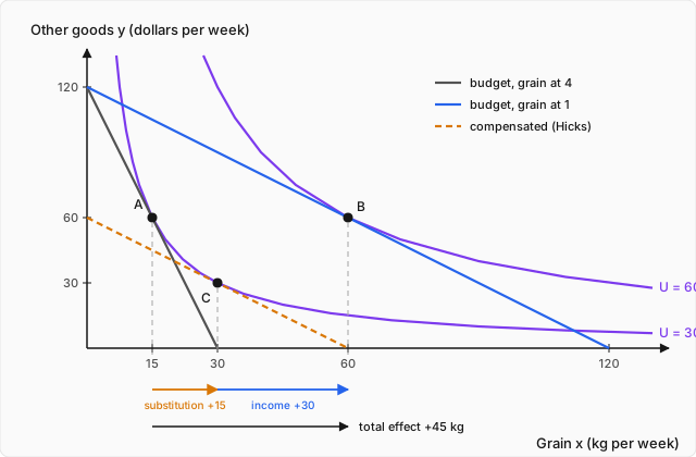
Rosa's household did exactly that. She had been buying 15 kilos a week; by the spring she was buying 60, and she was also spending more on everything else than she had before. Two doors down, the Bekele household did the reverse. They had been buying 15 kilos a week too, and after the price fell they bought 12. Less grain, at a quarter of the price, with no change in income, no change in the family, and no change in what they liked.

Nothing in the supply and demand apparatus can accommodate that. A demand curve slopes down; a lower price means a larger quantity demanded; the Bekeles are behaving like a counterexample to the first thing anyone learns. And the consumer choice topic, which built demand properly out of preferences and a budget constraint, did not obviously rule it out either. It ended by pointing at exactly this: when a price falls, two things happen to a consumer at once, and there is no law saying they push the same way.

Here is the split, stated before any algebra. When $p_x$ falls, grain becomes cheaper relative to everything else — the budget line pivots, the terms on which you can trade grain for other goods change, and the tangency condition $MRS = p_x/p_y$ now demands a different bundle. That is one change. But something else happened at the same instant: the bundle Rosa was already buying now costs less than it did, so she has money left over. She is, in the only sense that matters here, richer — not because anyone paid her, but because her income now commands more goods. That is a second change, and it has nothing to do with relative prices; it is the same thing that would have happened if grain had stayed at four dollars and someone had handed her cash.

Those two changes are the substitution effect and the income effect. They are not two events in time. Nobody substitutes on Monday and gets richer on Tuesday. They are two components of one movement, in the same sense that a diagonal step is not a step east followed by a step north — it is one step, which we choose to resolve into two perpendicular pieces because the pieces obey different laws. The substitution piece, as we will prove, always points toward the cheaper good. The income piece points wherever the good's income elasticity points, and for some goods that is backwards. When the backwards piece is bigger, you get the Bekeles.

Resolving one movement into two

Take a household with the preferences $u(x, y) = \sqrt{xy}$ , where $x$ is kilos of grain per week and $y$ is dollars spent on everything else, so that $p_y = 1$ by construction. Weekly income is $m = 120$ dollars. These are Cobb-Douglas preferences with equal exponents, so the demand functions derived in consumer choice apply directly with $\alpha = \beta = \tfrac12$ :

x^*(p_x, p_y, m) = \frac{1}{2}\frac{m}{p_x}, \qquad y^*(p_x, p_y, m) = \frac{1}{2}\frac{m}{p_y}.

Before the rail spur, $p_x = 4$ :

x_0 = \frac{1}{2}\cdot\frac{120}{4} = 15, \qquad y_0 = \frac{1}{2}\cdot\frac{120}{1} = 60,

and the bill checks: $4(15) + 60 = 120$ . ✓ Call that bundle $A = (15, 60)$ , with utility $u_0 = \sqrt{15 \times 60} = \sqrt{900} = 30$ .

After, $p_x = 1$ :

x_1 = \frac{1}{2}\cdot\frac{120}{1} = 60, \qquad y_1 = 60,

with $60 + 60 = 120$ ✓, giving bundle $B = (60, 60)$ and utility $u_1 = \sqrt{3600} = 60$ . The total effect on grain is $x_1 - x_0 = +45$ kilos.

Now the whole question of this topic: how much of that $+45$ is the pivot of the budget line, and how much is the fact that she got richer?

The trick, and it is the only trick in the subject, is to ask a counterfactual: what would she have bought at the new prices if we had simultaneously taken away just enough income to undo the enrichment? That hypothetical bundle sits between $A$ and $B$ . The move from $A$ to it is pure substitution — new relative prices, no change in how well off she is. The move from it to $B$ is pure income — no change in relative prices, only in how much she can afford.

Everything now rests on one phrase: just enough income to undo the enrichment. There are two defensible readings of it, they were proposed by two different people, and they give different numbers.

Hicks and Slutsky compensate differently

Hicks holds utility constant. Take away enough income that, facing the new prices, she can reach exactly her old indifference curve $u_0 = 30$ and no higher. Geometrically: slide the new budget line back, parallel to itself, until it is tangent to the original indifference curve.

Slutsky holds purchasing power over the original bundle constant. Take away enough income that, facing the new prices, she can just barely afford the exact bundle $A$ she used to buy. Geometrically: slide the new budget line back until it passes through the original point $A$ .

These sound like the same idea and are not. Compute both.

Hicks. We need the cheapest way to achieve $u = 30$ at prices $(p_x, p_y) = (1, 1)$ . That is the expenditure-minimization problem dual to the utility maximization already done, and for $u = \sqrt{xy}$ it has a clean solution. Minimize $p_x x + p_y y$ subject to $\sqrt{xy} = u$ ; the tangency condition is the same $MRS = p_x/p_y$ as before, and $MRS = y/x$ here, so $y = (p_x/p_y)x$ . Substituting into the constraint,

u = \sqrt{x \cdot \frac{p_x}{p_y}x} = x\sqrt{\frac{p_x}{p_y}} \quad\Longrightarrow\quad x^h(p_x, p_y, u) = u\sqrt{\frac{p_y}{p_x}}, \qquad y^h = u\sqrt{\frac{p_x}{p_y}}.

These are the Hicksian, or compensated, demand functions: quantity as a function of prices and a utility target, with no income argument at all. The minimized cost is the expenditure function

e(p_x, p_y, u) = p_x x^h + p_y y^h = u\sqrt{p_x p_y} + u\sqrt{p_x p_y} = 2u\sqrt{p_x p_y}.

Sanity check at the old prices: $e(4, 1, 30) = 2(30)(2) = 120$ , exactly her income — as it must be, since $A$ was her optimum. ✓ And $x^h(4,1,30) = 30\sqrt{1/4} = 15 = x_0$ ✓.

At the new prices, reaching $u_0 = 30$ costs

e(1, 1, 30) = 2(30)(1) = 60 \text{ dollars}.

So the Hicks-compensated income is 60 — the rail spur made her old standard of living cost half what it used to. At that income and those prices she would buy

x^H = x^h(1,1,30) = 30, \qquad y^H = 30,

which is bundle $C = (30, 30)$ , with $\sqrt{30 \times 30} = 30 = u_0$ ✓ and cost $30 + 30 = 60$ ✓. The Hicks decomposition is therefore

\underbrace{15 \to 30}_{\text{substitution } +15} \qquad \underbrace{30 \to 60}_{\text{income } +30} \qquad \underbrace{15 \to 60}_{\text{total } +45}. \;\checkmark

Slutsky. Now ask instead what the old bundle $A = (15, 60)$ costs at the new prices:

p^1 \cdot x_0 = 1(15) + 1(60) = 75 \text{ dollars}.

Give her 75 rather than 60 and let her choose freely. Cobb-Douglas demand at $(1, 1, 75)$ gives

x^S = \frac{1}{2}\cdot\frac{75}{1} = 37.5, \qquad y^S = 37.5,

so the Slutsky decomposition is

\underbrace{15 \to 37.5}_{\text{substitution } +22.5} \qquad \underbrace{37.5 \to 60}_{\text{income } +22.5} \qquad \underbrace{15 \to 60}_{\text{total } +45}. \;\checkmark

Same total, as it has to be — the endpoints $A$ and $B$ are facts about behavior, not about our bookkeeping. But the split is different: Hicks says $15/30$ , Slutsky says $22.5/22.5$ . That is not a rounding disagreement; the substitution effect under Slutsky is half again as large.

Which one is bigger is not an accident of this example, and the argument is worth having in general. The old bundle $x_0$ is one way of achieving the old utility $u_0$ at the new prices — she can always just buy it again. The Hicks compensation buys the cheapest way. So

e(p^1, u_0) \;\le\; p^1 \cdot x_0,

with equality only if the old bundle happens to be the cheapest route to $u_0$ at the new prices, which happens only when the prices have not actually changed. Slutsky compensation is always at least as generous as Hicks compensation (here, 75 against 60), so the Slutsky substitution effect is always at least as large. Notice also that a Slutsky-compensated consumer is strictly better off than she was: she can afford $A$ and, since relative prices moved, she can do better than $A$ — indeed $\sqrt{37.5 \times 37.5} = 37.5 > 30$ . Slutsky's construction deliberately does not hold welfare constant. Its compensation is to keep the old basket buyable, which is exactly what a cost-of-living index does when it prices a fixed basket, and that is not a coincidence.

The gap between them is large here only because the price change is huge — a factor of four. Shrink it and the two constructions converge: for a small change $dp_x$ , the difference between "afford the old bundle" and "reach the old utility" is second order, and the two substitution effects agree in the limit. That is why the Slutsky equation derived below can be written once and quoted by both camps.

The Hicks decomposition of a fall in the price of grain from 4 dollars to 1. The dashed amber line is the new budget line pushed back, parallel to itself, until it is just tangent to the original indifference curve — so the consumer at C is exactly as well off as she was at A but faces the new relative prices. The move from A to C is pure substitution and the move from C to B is pure income. Slutsky would instead push the line back only until it passed through A itself, which would put the intermediate bundle at 37.5 kilos rather than 30.

The Slutsky equation

The decomposition so far is arithmetic on two bundles. To say anything general — in particular, to say which way each piece must point — we need it in derivative form, for an arbitrary utility function.

Start from an identity that is almost a tautology once you read it slowly. At the utility level $u_0$ and prices $p$ , the cheapest bundle reaching $u_0$ costs $e(p, u_0)$ . A consumer handed exactly that much income and facing those prices will choose exactly that bundle — maximizing utility subject to a budget of $e(p,u_0)$ gets you back to the same point as minimizing expenditure subject to a utility target of $u_0$ . So for every price vector,

x^h(p, u_0) \;\equiv\; x^*\!\left(p,\; e(p, u_0)\right).

This holds identically in $p$ , so we may differentiate both sides with respect to $p_x$ . The right-hand side has $p_x$ in two places — directly, and inside the income argument — so the chain rule gives

\frac{\partial x^h}{\partial p_x} = \frac{\partial x^*}{\partial p_x} + \frac{\partial x^*}{\partial m}\cdot\frac{\partial e}{\partial p_x}.

The last factor is where the content is. Shephard's lemma says $\dfrac{\partial e}{\partial p_x} = x^h$ : the rate at which the minimum cost of a fixed standard of living rises with the price of $x$ is simply the quantity of $x$ being bought. That is the envelope theorem applied to the expenditure-minimization problem — when $p_x$ ticks up by $dp_x$ , the consumer re-optimizes, but the re-optimization is a second-order adjustment around a point where the first-order conditions already hold, so to first order the bill rises by (quantity) $\times$ $dp_x$ and nothing else. Our example obliges: $e = 2u\sqrt{p_xp_y}$ gives $\partial e/\partial p_x = u\sqrt{p_y/p_x} = x^h$ exactly. ✓

Substituting, and using $x^h = x^*$ at the point where the compensation is evaluated:

\boxed{\;\frac{\partial x^*}{\partial p_x} \;=\; \underbrace{\left.\frac{\partial x^h}{\partial p_x}\right|_{u = u_0}}_{\text{substitution effect}} \;-\; \underbrace{x\,\frac{\partial x^*}{\partial m}}_{\text{income effect}}\;}

This is the Slutsky equation. It says the observable response of demand to price — the slope of the demand curve you could in principle measure — is the sum of two unobservable pieces, one of which has a guaranteed sign.

The substitution term is never positive. This is a theorem, not an assumption, and it needs no calculus at all. Let $x^h(p)$ and $x^h(p')$ be the cost-minimizing bundles for the same utility level $u_0$ at two price vectors. Each minimizes cost at its own prices among bundles delivering $u_0$ , and the other bundle also delivers $u_0$ , so it was available and not chosen:

p \cdot x^h(p) \le p \cdot x^h(p'), \qquad p' \cdot x^h(p') \le p' \cdot x^h(p).

Add the two inequalities and collect terms:

(p - p')\cdot\left(x^h(p) - x^h(p')\right) \le 0.

Now let $p$ and $p'$ differ in the price of $x$ alone. Every other coordinate of $(p - p')$ is zero, so the whole dot product collapses to one term:

(p_x - p_x')\left(x^h_x(p) - x^h_x(p')\right) \le 0.

A price change and the compensated quantity change it produces always have opposite signs. Compensated demand curves slope downward, always, for every good, with no exceptions and no assumptions beyond consistent cost minimization. Check it on our formula: $x^h = u\,p_y^{1/2}p_x^{-1/2}$ , so $\partial x^h/\partial p_x = -\tfrac12 u\,p_y^{1/2}p_x^{-3/2} < 0$ everywhere. ✓

The income term is signed by the good, not by the theory. Its sign is the sign of $\partial x^*/\partial m$ , and the minus sign in front means: if $x$ is normal ( $\partial x^*/\partial m > 0$ ), the income term reinforces the substitution term — cheaper good, richer consumer, more of it, twice over. If $x$ is inferior ( $\partial x^*/\partial m < 0$ ), the income term opposes the substitution term, because being effectively richer makes her want less of it.

Verify the whole equation numerically at the original point, $p_x = 4$ , $p_y = 1$ , $m = 120$ , $x = 15$ , $u_0 = 30$ :

\frac{\partial x^*}{\partial p_x} = -\frac{m}{2p_x^2} = -\frac{120}{32} = -3.75,

\left.\frac{\partial x^h}{\partial p_x}\right|_{u_0} = -\frac{1}{2}(30)(1)\,4^{-3/2} = -\frac{15}{8} = -1.875, \qquad x\frac{\partial x^*}{\partial m} = 15\cdot\frac{1}{2p_x} = \frac{15}{8} = 1.875,

and indeed $-1.875 - 1.875 = -3.75$ . ✓ Two independently computed pieces reproducing a third.

One more form of the equation is worth having, because it is the one that connects to the vocabulary of elasticity. Multiply the Slutsky equation through by $p_x/x$ , and rewrite the income term by inserting $m/m$ :

\frac{p_x}{x}\frac{\partial x^*}{\partial p_x} = \frac{p_x}{x}\frac{\partial x^h}{\partial p_x} - p_x\frac{\partial x^*}{\partial m} = \frac{p_x}{x}\frac{\partial x^h}{\partial p_x} - \frac{p_x x}{m}\cdot\frac{m}{x}\frac{\partial x^*}{\partial m},

which in the standard names is

\varepsilon_p = \varepsilon_p^{\,h} - s_x\,\varepsilon_m,

where $s_x = p_x x/m$ is the budget share of $x$ and $\varepsilon_m$ its income elasticity. In our example $\varepsilon_p = -1$ (Cobb-Douglas demand is unit-elastic), $\varepsilon^h_p = -\tfrac12$ , $s_x = 60/120 = \tfrac12$ , and $\varepsilon_m = 1$ , giving $-\tfrac12 - \tfrac12(1) = -1$ . ✓ The budget share is the amplifier: a price change to a good you barely buy cannot make you meaningfully richer, no matter how inferior the good is.

Three cases, one of which is famous

The elasticity form makes the taxonomy exact. Since $\varepsilon^h_p \le 0$ always:

Normal good ( $\varepsilon_m > 0$ ): both terms are negative, $\varepsilon_p < 0$ . Demand slopes down, and more steeply than the compensated curve.
Inferior good ( $\varepsilon_m < 0$ ): the terms fight. Demand still slopes down as long as $|s_x\varepsilon_m| < |\varepsilon^h_p|$ — which is the usual case, because most inferior goods are small budget items.
Giffen good: the income term wins outright. Demand slopes up.

Written out, the Giffen condition is

\varepsilon_p > 0 \quad\Longleftrightarrow\quad s_x\varepsilon_m < \varepsilon^h_p \quad\Longleftrightarrow\quad \varepsilon_m < \frac{\varepsilon^h_p}{s_x} < 0.

Read the requirements off the right-hand inequality, because they are demanding. The good must be inferior ( $\varepsilon_m < 0$ ) — necessary, not sufficient. It must take a large budget share, since a small $s_x$ makes $\varepsilon^h_p/s_x$ hugely negative and puts the threshold out of reach. And it must have a weak substitution effect — few good substitutes, so $|\varepsilon^h_p|$ is small. A good that is simultaneously cheap-per-calorie, inferior, a large share of spending, and hard to substitute away from is a staple food eaten by people who are poor. Nothing else fits the profile.

Now the Bekeles. Their situation is close to a caricature, which is what makes it computable. They need 20 units of calories a week and no fewer. Grain delivers one unit per kilo at price $p_x$ ; meat delivers one unit per kilo at $p_y = 6$ . Meat is what they would rather eat, so within the set of calorie-adequate affordable bundles they take as much meat as they can. Income is $m = 60$ dollars a week.

With the calorie constraint binding, $x = 20 - y$ , and the budget gives

p_x(20 - y) + 6y = 60 \quad\Longrightarrow\quad y = \frac{60 - 20p_x}{6 - p_x}, \qquad x = 20 - y.

Before the rail spur, $p_x = 2$ :

y = \frac{60 - 40}{4} = 5, \qquad x = 15,

costing $2(15) + 6(5) = 30 + 30 = 60$ ✓ and delivering exactly 20 units of calories ✓. After, $p_x = 1$ :

y = \frac{60 - 20}{5} = 8, \qquad x = 12,

costing $12 + 48 = 60$ ✓, calories again exactly 20 ✓. Grain got cheaper and they bought less of it, 15 kilos down to 12 — which is what Rosa's neighbors could not explain.

Nothing irrational happened. Cheap grain was their way of hitting the calorie floor on a budget that could not otherwise reach it. When grain got cheaper, the floor became cheaper to clear, freeing money for the meat they actually wanted — and every kilo of meat bought replaces a kilo of grain, because the calorie requirement is already met. The decomposition confirms it: to hold their well-being fixed we would have to leave them buying $(15, 5)$ , which at the new prices costs $15 + 30 = 45$ dollars. At an income of 45 they buy exactly $(15, 5)$ again, so the substitution effect is zero, and the entire $-3$ kilos is income effect. Slutsky's equation, filled in: $\varepsilon^h_p = 0$ , $s_x = 30/60 = 0.5$ , and $\varepsilon_m = \frac{\partial x}{\partial m}\frac{m}{x} = \left(-\tfrac14\right)\frac{60}{15} = -1$ , so

\varepsilon_p = 0 - (0.5)(-1) = +0.5 > 0. \;\checkmark

Confirm it straight from the demand function: $\dfrac{\partial x}{\partial p_x} = -\dfrac{\partial y}{\partial p_x} = -\dfrac{-20(6-p_x) + (60-20p_x)}{(6-p_x)^2} = \dfrac{60}{16} = 3.75$ at $p_x = 2$ , and $\varepsilon_p = 3.75 \times \tfrac{2}{15} = +0.5$ . ✓

Be honest about what this model is. The rigid calorie constraint sets the substitution effect to exactly zero, which is the easiest possible way to get a Giffen good and is not how real preferences work; a genuine Giffen good needs the income term to overturn a strictly negative substitution term, which is harder. And the empirical record is thinner than the textbooks imply. The Irish potato story — routinely attributed to Robert Giffen, who never published it — has been examined against the actual famine data and does not hold up well; potato consumption fell. A 2008 field experiment in Hunan and Gansu, which randomized rice and wheat subsidies to poor households, reported Giffen behavior for staples among the very poor but not the poorest (who were too close to the floor to substitute at all), and its interpretation has been argued over since. The correct position is that the Slutsky equation permits Giffen goods, that the conditions it requires are severe and identifiable, and that whether any particular historical episode was one is a live empirical question rather than a settled fact.

An honest word about Cobb-Douglas

Look back at what happened to $y$ in the main example. Before: $y_0 = 60$ . After: $y_1 = 60$ . The price of grain fell by 75% and spending on everything else did not move by a cent.

That is not a deep truth about consumers; it is a property of the functional form. Cobb-Douglas demand $y^* = \frac{\beta}{\alpha + \beta}\frac{m}{p_y}$ contains no $p_x$ at all, so the cross-price effect $\partial y/\partial p_x$ is identically zero. Cobb-Douglas is therefore the worst possible example for illustrating substitution between goods, which is unfortunate, because it is the example everyone uses — including this topic, for its clean algebra.

The components do move, even when the total does not, and the decomposition shows it. Under the Hicks split, $y$ goes $60 \to 30$ from $A$ to $C$ (substitution: grain became relatively cheaper, so she moves toward grain and away from other goods) and then $30 \to 60$ from $C$ to $B$ (income: other goods are normal, so the compensation returned buys more of them). The two are exactly equal and opposite. Cobb-Douglas is the knife edge, and the knife edge has an interpretation: its elasticity of substitution is exactly 1, which is precisely the value at which the substitution and income effects on the other good cancel.

Step off the knife edge and the cross effect reappears with either sign. Take CES preferences $u = (x^\rho + y^\rho)^{1/\rho}$ , whose demands are $x^* = \dfrac{p_x^{-\sigma}}{p_x^{1-\sigma} + p_y^{1-\sigma}}m$ with elasticity of substitution $\sigma = 1/(1-\rho)$ , and run the same price fall from 4 to 1 with $m = 120$ , $p_y = 1$ :

\begin{array}{l|rr|rr} & x \text{ at } p_x = 4 & y \text{ at } p_x = 4 & x \text{ at } p_x = 1 & y \text{ at } p_x = 1 \\ \hline \sigma = 2 \;(\rho = \tfrac12) & 6 & 96 & 60 & 60 \\ \sigma = 1 \;(\text{Cobb-Douglas}) & 15 & 60 & 60 & 60 \\ \sigma = \tfrac12 \;(\rho = -1) & 20 & 40 & 60 & 60 \end{array}

Every row satisfies the budget constraint exactly — check the top left: $4(6) + 96 = 120$ ✓, and $4(20) + 40 = 120$ ✓. With $\sigma = 2$ the goods substitute easily and cheap grain cannibalizes other spending, $96 \to 60$ . With $\sigma = \tfrac12$ they are hard to substitute, the income effect dominates the cross relationship, and other spending rises, $40 \to 60$ . Cobb-Douglas sits exactly between, at zero, which is the one case that teaches nothing about the mechanism.

Two demand curves, and which one is the real one

We now have two demand functions for the same consumer and the same good, and they are not the same curve.

\text{Marshallian (ordinary): } x^*(p_x) = \frac{60}{p_x}, \qquad \text{Hicksian (compensated) at } u_0 = 30: \; x^h(p_x) = \frac{30}{\sqrt{p_x}}.

They agree at $p_x = 4$ , where both give 15 — by construction, since that is the price at which the compensation is zero. Away from it they diverge:

\begin{array}{r|rrrr} p_x & 1 & 2 & 4 & 9 \\ \hline x^*(p_x) & 60 & 30 & 15 & 6.\overline{6} \\ x^h(p_x) & 30 & 21.2 & 15 & 10 \end{array}

The compensated curve is flatter in quantity and therefore steeper as a curve drawn with price on the vertical axis: it moves less, in both directions. The reason is the Slutsky equation read backwards. The ordinary curve contains both effects; the compensated curve contains only the substitution effect. For a normal good the two effects point the same way, so stripping out the income effect leaves less movement. Their slopes at the common point make it exact: $-3.75$ against $-1.875$ , or in elasticities, $-1$ against $-\tfrac12$ . For an inferior good the ordering flips — the income effect was working against the substitution effect, so removing it leaves more movement, and the compensated curve is the flatter one.

Which curve you want depends on the question. If you want to predict how much grain gets bought, you want the ordinary curve, because that is what people actually do. If you want to measure how much better off the price cut made Rosa, you want a compensated curve — and this is where the topic pays off a debt to consumer surplus.

That topic measured the gain from a price fall as the area to the left of the demand curve between the two prices. Do that here:

\Delta CS = \int_1^4 \frac{60}{p}\,dp = 60\ln 4 \approx 83.18 \text{ dollars}.

Now compute the two answers that are actually defensible. The compensating variation is the money we could take away from Rosa after the price fall to leave her exactly as well off as before — which is exactly the Hicks compensation already computed:

CV = m - e(p^1, u_0) = 120 - 60 = 60 \text{ dollars},

and it is also the area under the compensated curve through $u_0$ :

\int_1^4 30\,p^{-1/2}dp = 60\left[\sqrt{p}\,\right]_1^4 = 60(2 - 1) = 60. \;\checkmark

The equivalent variation is the money we would have had to give her instead of the price fall to make her equally happy:

EV = e(p^0, u_1) - m = 2(60)(2) - 120 = 240 - 120 = 120 \text{ dollars},

which is likewise the area under the compensated curve through the new utility level, $\int_1^4 60p^{-1/2}dp = 120$ . ✓ So

CV = 60 \;\le\; \Delta CS \approx 83.18 \;\le\; EV = 120,

the ordinary consumer surplus sitting between the two Hicksian measures — always, for a normal good and a price fall, because the ordinary demand curve lies between the two compensated curves. The gap here is embarrassing: the surplus number overstates the compensating variation by 39%. That is because this price change is enormous. For modest price changes, and goods with modest budget shares, the three collapse toward each other fast — the error is second order in both the price change and the income effect — which is why the surplus triangles of the earlier topics are a legitimate working tool and not a fraud. But when you are evaluating a tax on a staple that eats a third of a household's budget, the distinction is the whole answer.

Worked example

A household has preferences $u(x,y) = x^{1/3}y^{2/3}$ , income $m = 96$ dollars a week, and faces $p_y = 2$ . The price of $x$ falls from 8 to 1. (a) Find the old and new optimal bundles and the total effect on $x$ . (b) Decompose it the Hicks way, verifying that the intermediate bundle really delivers the original utility. (c) Decompose it the Slutsky way. (d) Which substitution effect is larger, and why must it be? (e) Verify the Slutsky equation numerically at the original prices. (click to reveal the solution)

Setting up. For $u = x^\alpha y^\beta$ the demand functions established in consumer choice are $x^* = \frac{\alpha}{\alpha+\beta}\frac{m}{p_x}$ and $y^* = \frac{\beta}{\alpha+\beta}\frac{m}{p_y}$ . Here $\alpha = \tfrac13$ , $\beta = \tfrac23$ , so the shares are $\tfrac13$ and $\tfrac23$ :

x^* = \frac{1}{3}\frac{m}{p_x}, \qquad y^* = \frac{2}{3}\frac{m}{p_y}.

Step (a) — the two optima. At $p_x = 8$ :

x_0 = \frac{1}{3}\cdot\frac{96}{8} = 4, \qquad y_0 = \frac{2}{3}\cdot\frac{96}{2} = 32,

with bill $8(4) + 2(32) = 32 + 64 = 96$ ✓. Utility:

u_0 = 4^{1/3}\,32^{2/3} = \left(4 \cdot 32^2\right)^{1/3} = \left(4 \cdot 1024\right)^{1/3} = 4096^{1/3} = 16.

At $p_x = 1$ :

x_1 = \frac{1}{3}\cdot 96 = 32, \qquad y_1 = 32,

bill $32 + 64 = 96$ ✓, and $u_1 = 32^{1/3}32^{2/3} = 32$ . Total effect on $x$ : $+28$ .

Step (b) — Hicks. Derive the compensated demand from scratch. Minimizing $p_xx + p_yy$ subject to $x^{1/3}y^{2/3} = u$ gives the same tangency as before, $MRS = \frac{\alpha}{\beta}\frac{y}{x} = \frac{p_x}{p_y}$ , so

\frac{1}{2}\frac{y}{x} = \frac{p_x}{p_y} \quad\Longrightarrow\quad y = \frac{2p_x}{p_y}x.

Substitute into the utility target:

u = x^{1/3}\left(\frac{2p_x}{p_y}x\right)^{2/3} = x\left(\frac{2p_x}{p_y}\right)^{2/3} \quad\Longrightarrow\quad x^h = u\left(\frac{p_y}{2p_x}\right)^{2/3}.

Check it reproduces the old optimum: at $p_x = 8$ , $p_y = 2$ , $u = 16$ , the bracket is $\left(\frac{2}{16}\right)^{2/3} = (1/8)^{2/3} = 1/4$ , so $x^h = 16/4 = 4 = x_0$ ✓.

Now hold $u = 16$ and impose the new prices, $p_x = 1$ , $p_y = 2$ . The bracket is $\left(\frac{2}{2}\right)^{2/3} = 1$ , so

x^H = 16, \qquad y^H = \frac{2(1)}{2}(16) = 16.

Verify the utility really is unchanged, which is the whole point of the Hicks construction: $16^{1/3}16^{2/3} = 16 = u_0$ ✓. The compensated income is the cost of that bundle at the new prices, $1(16) + 2(16) = 48$ dollars — half her actual income, which the general formula $e = u\left(\frac{p_x}{\alpha}\right)^{\alpha}\left(\frac{p_y}{\beta}\right)^{\beta} = u(3p_x)^{1/3}(3p_y)^{2/3}$ confirms: at $(8,2)$ it gives $16(24)^{1/3}(6)^{2/3} = 16(24 \cdot 36)^{1/3} = 16(864)^{1/3}$ . Since $864 = 216 \cdot 4$ , this is $16 \cdot 6 \cdot 4^{1/3}$ — not 96, so the formula as written is wrong; the correct grouping is $e = u\left(\frac{p_x}{\alpha}\right)^{\alpha}\left(\frac{p_y}{\beta}\right)^{\beta} = u(3p_x)^{1/3}\left(\tfrac{3}{2}p_y\right)^{2/3}$ , giving $16(24)^{1/3}(3)^{2/3} = 16(216)^{1/3} = 16(6) = 96$ ✓, and at $(1,2)$ , $16(3)^{1/3}(3)^{2/3} = 16(3) = 48$ ✓. So:

\underbrace{4 \to 16}_{\text{substitution } +12}, \qquad \underbrace{16 \to 32}_{\text{income } +16}, \qquad \text{total } +28. \;\checkmark

Step (c) — Slutsky. Price the original bundle $(4, 32)$ at the new prices:

p^1\cdot x_0 = 1(4) + 2(32) = 68 \text{ dollars}.

Hand her 68 and let her choose freely at the new prices:

x^S = \frac{1}{3}\cdot\frac{68}{1} = \frac{68}{3} = 22\tfrac{2}{3}, \qquad y^S = \frac{2}{3}\cdot\frac{68}{2} = \frac{68}{3} = 22\tfrac{2}{3},

and the bill is $\tfrac{68}{3} + 2\cdot\tfrac{68}{3} = 68$ ✓. So

\underbrace{4 \to \tfrac{68}{3}}_{\text{substitution } +\tfrac{56}{3} = 18\tfrac{2}{3}}, \qquad \underbrace{\tfrac{68}{3} \to 32}_{\text{income } +\tfrac{28}{3} = 9\tfrac{1}{3}}, \qquad \text{total } \tfrac{56}{3} + \tfrac{28}{3} = \tfrac{84}{3} = 28. \;\checkmark

Note also that the Slutsky-compensated household reaches utility $\left(\tfrac{68}{3}\right)^{1/3}\left(\tfrac{68}{3}\right)^{2/3} = \tfrac{68}{3} \approx 22.7 > 16$ : strictly better off than before, as Slutsky compensation always leaves a consumer after a price change.

Step (d) — why Slutsky's is larger. $18\tfrac23 > 12$ , and it had to be. Slutsky left her 68 dollars; Hicks left her 48. The old bundle $(4,32)$ is a way of reaching $u_0 = 16$ at the new prices, and Hicks buys the cheapest way, so $e(p^1, u_0) \le p^1\cdot x_0$ — here $48 \le 68$ . More income at the same new prices means more $x$ , since $x$ is normal, so the intermediate bundle sits further right under Slutsky and the substitution effect it measures is larger. This ordering is general for any price change and any preferences: the Slutsky substitution effect is never smaller in magnitude than the Hicks one, and the two coincide only in the limit of an infinitesimal price change.

Step (e) — the Slutsky equation at $p_x = 8$ . The three derivatives, each computed independently. Ordinary:

\frac{\partial x^*}{\partial p_x} = -\frac{m}{3p_x^2} = -\frac{96}{3(64)} = -\frac{1}{2}.

Compensated, from $x^h = u\left(\frac{p_y}{2}\right)^{2/3}p_x^{-2/3}$ :

\frac{\partial x^h}{\partial p_x} = -\frac{2}{3}\,\frac{x^h}{p_x} = -\frac{2}{3}\cdot\frac{4}{8} = -\frac{1}{3}.

Income:

x\frac{\partial x^*}{\partial m} = 4 \cdot \frac{1}{3p_x} = \frac{4}{24} = \frac{1}{6}.

Assemble: $-\tfrac13 - \tfrac16 = -\tfrac12$ ✓. And in elasticity form, $\varepsilon_p = -1$ , $\varepsilon^h_p = -\tfrac23$ , $s_x = 32/96 = \tfrac13$ , $\varepsilon_m = 1$ , so $-\tfrac23 - \tfrac13(1) = -1$ ✓. The compensated elasticity $-\tfrac23$ is exactly $-(1-\alpha)$ , and the budget share is exactly $\alpha$ — a Cobb-Douglas signature worth remembering.

One last observation. Track $y$ through the Hicks decomposition: $32 \to 16 \to 32$ . Total change zero, components $\pm 16$ . The good whose price never changed was pushed hard in both directions and ended exactly where it started — a reminder that "no effect" and "no effects" are different statements.

Where this leads

One price change, two components. The substitution component is signed by a theorem that needs nothing but consistent cost minimization; the income component is signed by whether the good is normal or inferior; and the Slutsky equation

\frac{\partial x}{\partial p_x} = \left.\frac{\partial x^h}{\partial p_x}\right|_{U} - x\frac{\partial x}{\partial m}

is the accounting identity that holds them together. Hicks and Slutsky answer the same question with two different definitions of "as well off as before", differ by a second-order amount for small price changes, and differ by 50% here because the price moved by a factor of four. Giffen goods are exactly the case where an inferior good with a large budget share and few substitutes lets the income term win — permitted by the equation, rare in the world, and much less settled empirically than the potato anecdote suggests.

This machinery is the reason the consumer surplus triangles have to be treated as approximations rather than measurements. When a government taxes a staple, the honest question is not "how much smaller is the triangle" but "how many dollars would we have to hand this household to leave it as well off as before the tax", and that number — the compensating variation — is an area under a curve nobody can observe directly. Every applied welfare number you will ever see, from the burden of a carbon tax to the gain from a trade agreement, is somebody's attempt to recover a Hicksian object from Marshallian data. The deadweight loss computed earlier was, strictly, the Marshallian version of a Hicksian idea. It is worth knowing which one you are holding.

The natural next step is to notice how much of this survives aggregation, and how much does not. Two things are guaranteed for a single consumer: her compensated demand slopes down, and — a fact we derived without noticing — the cross-substitution effects are symmetric, since $\partial x^h/\partial p_y = \partial^2 e/\partial p_y \partial p_x = \partial y^h/\partial p_x$ by the equality of mixed partials on the expenditure function. That symmetry is a strong, testable restriction on real demand data, and it is the reason economists can go backwards from observed behavior to preferences at all.

But add up a thousand households, each individually well behaved, and the guarantee weakens in a way that is genuinely surprising the first time you meet it: market demand need not inherit the properties of individual demand, because a price change redistributes real income across people with different tastes. The substitution effects still all point the right way; the income effects no longer cancel neatly. What is left of the theory once every price in the economy is allowed to move at once — and whether the resulting equilibrium can still be called efficient in the sense the surplus topic claimed — is the subject of general equilibrium and the welfare theorems. Bring the Slutsky equation with you; the second welfare theorem is, at bottom, an argument about income effects.

Check yourself