Electric Potential and Potential Energy

Go back to the ball rolling down the frictionless hill in work and energy. The whole point of that topic was that you never had to track the hill's shape, or the normal force at each instant, or any moment of the trip in between — a single number, potential energy, evaluated at the start and the end, told you everything about the speed. That was possible because gravity is a conservative force. Coulomb's law gives you a force between charges that has exactly the same inverse-square shape as gravity between masses — so it's worth asking, seriously, whether the same shortcut is available here too. It is, and chasing it down gives you one of the single most useful quantities in all of electromagnetism.

Is the electric force actually conservative?

Vector calculus proved something exact and general: a force is conservative if and only if its curl vanishes everywhere,

\vec F \text{ is conservative} \iff \nabla\times\vec F = \vec 0.

The electric field of a point charge, $\vec E = k\dfrac{q}{r^2}\hat r$ , points radially outward (or inward) from the charge at every location, with a magnitude that depends only on distance $r$ . A field like this — purely radial, with no angular dependence — has zero curl everywhere except possibly at the source point itself; there is nothing for an imaginary paddle wheel to catch, since the field never has a component that circulates around any point off the radial line through the charge. (This can be checked directly by computing $\nabla\times\vec E$ in spherical coordinates and finding it vanishes identically — a calculation this topic won't carry out in full, but the qualitative picture, and the exact statement from the vector calculus topic, are enough to trust the conclusion.) So the electric force is conservative, for the same structural reason gravity is, and the vector calculus theorem guarantees something powerful follows immediately: the electric field can be written as the gradient of a scalar potential.

Defining electric potential

Exactly as work and energy defined a potential energy $U$ for any conservative force via $\vec F = -\nabla U$ , define the electric potential $V$ by dividing the electric potential energy $U$ of a test charge $q_0$ by the charge itself:

V \equiv \frac{U}{q_0}.

This is the same conceptual move Coulomb's law made to get from force to field: force per unit charge gave the field $\vec E$ ; potential energy per unit charge gives the potential $V$ . And exactly as $\vec E$ turned out to be a property of the space around a charge, independent of whether any test charge was actually there to feel it, $V$ is too — a number assigned to every point in space, waiting to be multiplied by whatever charge you place there to get that charge's potential energy back: $U = q_0 V$ . Potential is measured in joules per coulomb, a combination given its own name, the volt (V).

From potential back to field: $\vec E = -\nabla V$

Divide both sides of $\vec F = -\nabla U$ by the test charge $q_0$ :

\frac{\vec F}{q_0} = -\nabla\left(\frac{U}{q_0}\right).

The left side is exactly the definition of the electric field, $\vec E = \vec F/q_0$ . The right side, using $V = U/q_0$ , is $-\nabla V$ . So:

\vec E = -\nabla V.

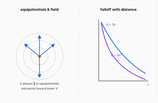
This is worth pausing on, because it compresses an enormous amount of physics into three symbols. The electric field — a full vector, three numbers at every point in space — can be recovered completely by knowing just one number at every point (the potential $V$ ) and differentiating it. All the directional information the field carries is really information about how $V$ changes from place to place: the field points in the direction $V$ decreases fastest (the minus sign), exactly as the gradient topic showed $-\nabla h$ is the direction water actually flows downhill. A positive test charge, released from rest, always accelerates toward lower potential — "downhill" on the potential landscape — the same way a ball released on a real hill rolls toward lower height.

The potential of a point charge

To find $V$ for a single point charge $q$ , use the same fundamental-theorem-of-gradients relation the integral theorems topic proved: $\int_C(\nabla f)\cdot d\vec l = f(\vec b) - f(\vec a)$ . Applied here (with a minus sign, since $\vec E=-\nabla V$ ), the potential difference between two points is minus the line integral of the field between them, and choosing the conventional reference point $V=0$ at $r=\infty$ (physically sensible, since a charge's influence should die away to nothing infinitely far from it) gives, after carrying out the integral along a radial path from $\infty$ in to a distance $r$ :

V(r) = k\frac{q}{r}.

Notice the exponent: force and field fell off as $1/r^2$ , but potential falls off only as $1/r$ — one power of $r$ gentler, exactly as expected from the fact that $V$ is built by integrating the field over distance, and integration is the inverse of the differentiation that would turn $1/r$ back into $1/r^2$ . For a system of several point charges, potential obeys the same superposition principle the field does — but with a genuine simplification: potentials are ordinary numbers, not vectors, so combining the potential from several charges at a point is just ordinary addition, no components, no angles, no trigonometry required.

Two panels. Left: a single positive point charge with concentric dashed circles around it labeled as equipotential surfaces, and a radial arrow labeled E pointing outward, perpendicular to the circles. Right: a graph of potential V against distance r for a point charge, a curve falling off as one over r, alongside a second curve falling off faster, as one over r squared, labeled E, for comparison.

Left: the field is everywhere perpendicular to surfaces of constant potential, pointing toward lower V. Right: potential falls off one power of r more gently than the field, because V is the field's integral.

Worked example

A charge $q_1 = +4.0\ \mu\text{C}$ sits at the origin, and a charge $q_2 = -2.0\ \mu\text{C}$ sits 3.0 m away. Find the electric potential at the midpoint between them, and the potential energy of a $+1.0\ \mu\text{C}$ test charge placed at that midpoint. (click to reveal the solution)

Setting up: the midpoint is $1.5$ m from each charge. Potential is a scalar, so the total potential at the midpoint is just the ordinary sum of the potential due to each charge separately — no vector components needed, which is exactly the simplification this topic promised over working with the field directly.

Potential from $q_1$ at distance $r_1 = 1.5$ m:

V_1 = k\frac{q_1}{r_1} = \frac{(8.99\times10^9)(4.0\times10^{-6})}{1.5} \approx 2.397\times10^4\ \text{V}.

Potential from $q_2$ at distance $r_2 = 1.5$ m, keeping the sign of $q_2$ (potential, unlike distance, can be negative):

V_2 = k\frac{q_2}{r_2} = \frac{(8.99\times10^9)(-2.0\times10^{-6})}{1.5} \approx -1.199\times10^4\ \text{V}.

Total potential at the midpoint, by superposition:

V = V_1 + V_2 \approx 2.397\times10^4 - 1.199\times10^4 \approx 1.20\times10^4\ \text{V}.

The result is positive — unsurprising, since the closer inspection shows the positive charge's contribution is larger in magnitude at equal distance simply because $|q_1| > |q_2|$ , and both are the same distance away.

Potential energy of the test charge, using $U = q_0 V$ with $q_0 = +1.0\times10^{-6}$ C:

U = q_0 V = (1.0\times10^{-6})(1.20\times10^4) \approx 1.20\times10^{-2}\ \text{J}.

Interpreting the result: the potential energy is positive, meaning it would take positive work to bring the test charge in from infinity to this point (or equivalently, the test charge would gain kinetic energy if released and allowed to fly back out to infinity, converting this stored $1.20\times10^{-2}$ J entirely into motion). Notice how little work this took compared to a full vector field calculation like the one in Coulomb's law's worked example: two plain numbers were added, with no angles, no components, and no trigonometry anywhere in sight — precisely the payoff potential is built to deliver.

Where this leads

Potential is what makes the electric field tractable for anything more complicated than a couple of point charges — instead of adding vectors, you add numbers, and then differentiate once at the end to recover the field if you need it. That trade — one scalar function standing in for a whole vector field — is about to become even more powerful once Gauss's law gives a second, often much faster way to find the field itself directly from symmetry, and once conductors and capacitance puts potential to work explaining why charge distributes itself on a conductor exactly the way it does.