Electric Current and Simple Circuits

Every topic in this track's electromagnetism branch so far has quietly assumed the charges involved have already finished moving and settled down — Coulomb's law and Gauss's law describe static arrangements, and even conductors and capacitance is really a story about charge redistributing once and then stopping. But the most useful thing you can do with charge is keep it moving, continuously and controllably — that's a flashlight, a phone, a heating element, the entire discipline of electronics. This topic is about what happens the moment "electrostatics" stops being an accurate word for the situation.

Current: how much charge, how fast

Define the electric current through a wire as the rate at which charge passes a given cross-section:

I \equiv \frac{dq}{dt},

measured in coulombs per second, a unit given its own name, the ampere (A). By historical convention fixed long before anyone knew electrons carry negative charge, current is defined as flowing in the direction positive charge would move — so in an ordinary metal wire, where the actual moving carriers are negatively charged electrons, the conventional current direction is opposite to the electrons' actual drift direction. This convention is a permanent minor annoyance, not a physical subtlety, and it's worth stating plainly once so it never causes confusion later: whenever this topic (or any other) says "current flows this way," it means positive-charge-equivalent flow, regardless of which sign the actual carriers happen to be.

For a wire with cross-sectional area $A$ , it's often useful to describe the flow at the level of a single point instead of an entire cross-section, using the current density $\vec J$ — current per unit area, pointing along the direction of flow — related to the total current by:

I = \int_A \vec J\cdot d\vec A.

For a uniform current spread evenly over a wire's cross-section, this simplifies to $I = JA$ .

Ohm's law: the simplest possible relationship between push and flow

Push charge through most ordinary materials — metals especially — and, over a wide range of conditions, the current that flows turns out to be directly proportional to the voltage applied:

V = IR.

This is Ohm's law, and $R$ , the resistance, is the constant of proportionality — a single number (measured in ohms, $\Omega$ ) summarizing how strongly a particular piece of material opposes the flow of current. It's worth being honest about the status of this equation: unlike $F=ma$ or Gauss's law, Ohm's law is not a fundamental law of physics derivable from first principles — it's an excellent empirical description of how many real materials actually behave, valid because the collisions between drifting charge carriers and the material's atoms produce, on average, a drag force proportional to drift speed, which itself is proportional to current. Some materials (semiconductors, diodes, anything used precisely because it doesn't obey Ohm's law) break this proportionality entirely, and even ordinary resistors stop obeying it if pushed to extremes of temperature or voltage. Where it holds, though, it holds extremely well, and it's the workhorse of everything in this topic.

Resistance itself depends on both the material a wire is made of and its geometry:

R = \rho\frac{L}{A},

where $L$ is the wire's length, $A$ its cross-sectional area, and $\rho$ (rho) is the resistivity — a property of the material alone, independent of its shape, playing a role for electrical conduction analogous to the role density plays for mass. Longer wires resist more (charge has to fight through more material); fatter wires resist less (more parallel "lanes" for current to flow through) — both matching the intuition you'd expect from, say, water flowing through a pipe of a given length and width.

Combining resistors: series and parallel

Resistors in series — connected end to end, so the same current $I$ must flow through each one in turn, with no other path available — divide the total voltage across the combination. The voltage across each resistor is $V_i = IR_i$ , and the total voltage is the sum:

V_{\text{total}} = V_1+V_2+\cdots = IR_1+IR_2+\cdots = I(R_1+R_2+\cdots).

Comparing to $V_{\text{total}} = IR_{\text{eq}}$ for a single equivalent resistor carrying the same current at the same total voltage:

R_{\text{eq}} = R_1+R_2+\cdots \qquad \text{(series)}.

Resistors in parallel — connected so that both ends of every resistor share the same two nodes, meaning each one sees the identical voltage $V$ across it, while the current splits between them — instead add up the currents. Each branch carries $I_i = V/R_i$ , and the total current entering the parallel combination is the sum of what flows through each branch:

I_{\text{total}} = I_1+I_2+\cdots = \frac{V}{R_1}+\frac{V}{R_2}+\cdots = V\left(\frac{1}{R_1}+\frac{1}{R_2}+\cdots\right).

Comparing to $I_{\text{total}} = V/R_{\text{eq}}$ :

\frac{1}{R_{\text{eq}}} = \frac{1}{R_1}+\frac{1}{R_2}+\cdots \qquad \text{(parallel)}.

Notice the pattern is a mirror image of how capacitors combine (a fact not derived here, but worth flagging): resistors in series add directly while parallel resistors add as reciprocals, exactly the opposite pattern from capacitance, because a capacitor's job (storing charge for a given voltage) and a resistor's job (opposing current for a given voltage) are, in a real sense, reciprocal functions of each other.

Kirchhoff's rules: conservation laws in disguise

Series and parallel combinations only get you so far — plenty of real circuits (multiple batteries, resistors that share nodes in more tangled ways) can't be reduced to a single equivalent resistor by combining series and parallel pieces alone. Kirchhoff's rules handle the general case, and both are really just conservation laws wearing circuit-diagram clothing, not new physics invented for the occasion.

The junction rule (charge conservation): at any point where wires meet — a junction or node — the total current flowing in must equal the total current flowing out.

\sum I_{\text{in}} = \sum I_{\text{out}}.

If this weren't true, charge would be piling up (or draining away) at that single point, forever, which conservation of charge — the same fact Coulomb's law opened with — flatly forbids in a steady-flowing circuit.

The loop rule (energy conservation): the sum of all potential changes — voltage rises from batteries, voltage drops across resistors — going all the way around any closed loop in a circuit must equal zero.

\sum_{\text{loop}} \Delta V = 0.

This is the electrical version of the fact from work and energy and electric potential that potential is a well-defined function of position — walk all the way around any closed loop back to your starting point, and whatever potential you started with, you must return to, so all the rises and drops along the way have to cancel exactly.

A two-loop resistor circuit with two batteries and three resistors. A left branch contains a battery labeled epsilon 1 and resistor R1 carrying current i1 downward, a right branch contains a battery labeled epsilon 2 and resistor R2 carrying current i2 downward, and a middle branch contains resistor R3 carrying current i3 upward, all three branches meeting at a top node a and bottom node b. — A circuit too tangled for series-parallel reduction alone: three branches, two batteries, solvable only by combining the junction rule (charge conservation) and the loop rule (energy conservation).

Worked example

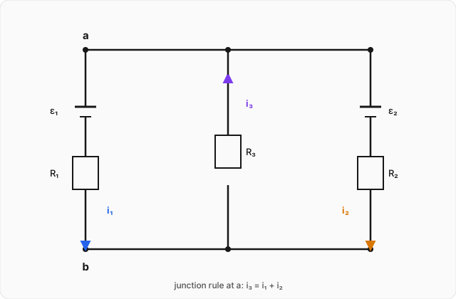
In the circuit shown, $\varepsilon_1 = 10\ \text{V}$ , $\varepsilon_2 = 5\ \text{V}$ , $R_1 = R_2 = 5\ \Omega$ , and $R_3 = 10\ \Omega$ . Find the current in each of the three branches. (click to reveal the solution)

Setting up: label the three branch currents $i_1$ (through $\varepsilon_1$ and $R_1$ , assumed flowing from node $a$ down to node $b$ ), $i_2$ (through $\varepsilon_2$ and $R_2$ , also assumed $a$ to $b$ ), and $i_3$ (through $R_3$ alone, assumed flowing from $b$ up to $a$ ). If any of these assumed directions turns out to be wrong, the algebra will simply hand back a negative number for that current — Kirchhoff's rules don't require guessing correctly, only guessing consistently.

Junction rule at node $a$ : current $i_3$ flows in; currents $i_1$ and $i_2$ flow out. So:

i_3 = i_1 + i_2. \qquad (1)

Loop rule, left loop (branch 1 and branch 3): traversing from $b$ up through $R_3$ to $a$ (against the assumed direction of $i_3$ , so this is a rise of $+i_3R_3$ ... more carefully: since $i_3$ is defined flowing $b\to a$ , traveling $b\to a$ with the current through a resistor is a voltage drop, $-i_3R_3$ ), then from $a$ down through branch 1 back to $b$ (through the battery, a rise of $\varepsilon_1$ , then through $R_1$ in the direction of $i_1$ , a drop of $i_1R_1$ ):

-i_3R_3 + \varepsilon_1 - i_1R_1 = 0 \quad\Longrightarrow\quad \varepsilon_1 = i_3R_3 + i_1R_1. \qquad (2)

Loop rule, right loop (branch 2 and branch 3), by the identical argument:

\varepsilon_2 = i_3R_3 + i_2R_2. \qquad (3)

Substituting numbers. With $R_1=R_2=5\ \Omega$ , $R_3=10\ \Omega$ , $\varepsilon_1=10\ \text{V}$ , $\varepsilon_2=5\ \text{V}$ , and using (1) to eliminate $i_3$ from (2) and (3):

10 = 10(i_1+i_2) + 5i_1 = 15i_1 + 10i_2, \qquad (2')

5 = 10(i_1+i_2) + 5i_2 = 10i_1 + 15i_2. \qquad (3')

Solving the simultaneous equations. Multiply (2 $'$ ) by 3 and (3 $'$ ) by 2:

45i_1 + 30i_2 = 30, \qquad 20i_1+30i_2=10.

Subtracting the second from the first eliminates $i_2$ :

25i_1 = 20 \quad\Longrightarrow\quad i_1 = 0.8\ \text{A}.

Substituting back into (2 $'$ ):

15(0.8) + 10i_2 = 10 \quad\Longrightarrow\quad 12 + 10i_2 = 10 \quad\Longrightarrow\quad i_2 = -0.2\ \text{A}.

And from (1):

i_3 = i_1+i_2 = 0.8 + (-0.2) = 0.6\ \text{A}.

Checking against equation (3 $'$ ) as an independent consistency check: $10(0.8)+15(-0.2) = 8-3=5$ , matching $\varepsilon_2=5$ exactly.

Interpreting the result: $i_1 = 0.8\ \text{A}$ and $i_3=0.6\ \text{A}$ came out positive, so the assumed directions for those two were correct. $i_2$ came out negative, $-0.2\ \text{A}$ , meaning the actual current in that branch runs opposite to what was assumed — from $a$ to $b$ , not $b$ to $a$ — physically sensible once you notice $\varepsilon_2$ is the weaker of the two batteries and finds itself fighting against the stronger $\varepsilon_1$ pushing current the other way through the shared branch $R_3$ . The algebra didn't need to be told this in advance; the sign handled it automatically.

Where this leads

Current and circuits round out the electrostatic and steady-current picture of electromagnetism this branch of the track has been building since Coulomb's law. The next real turn is a genuinely new phenomenon: a current — charge in motion — turns out to generate a completely different kind of field, one that pushes on other moving charges rather than stationary ones. That's magnetic field and force, and from there the track builds toward Biot-Savart and Ampère's law, Faraday's law of induction, and eventually Maxwell's equations — the complete, unified statement of everything electric and magnetic fields do, culminating in electromagnetic waves: the discovery that light itself is one of these fields, oscillating.